Summary of WP1 data products for FACE-IT study sites
Robert Schlegel
01 octobre 2024
Last updated: 2024-10-01
Checks: 7 0
Knit directory: WP1/
This reproducible R Markdown analysis was created with workflowr (version 1.7.1). The Checks tab describes the reproducibility checks that were applied when the results were created. The Past versions tab lists the development history.
Great! Since the R Markdown file has been committed to the Git repository, you know the exact version of the code that produced these results.
Great job! The global environment was empty. Objects defined in the global environment can affect the analysis in your R Markdown file in unknown ways. For reproduciblity it’s best to always run the code in an empty environment.
The command set.seed(20210216) was run prior to running
the code in the R Markdown file. Setting a seed ensures that any results
that rely on randomness, e.g. subsampling or permutations, are
reproducible.
Great job! Recording the operating system, R version, and package versions is critical for reproducibility.
Nice! There were no cached chunks for this analysis, so you can be confident that you successfully produced the results during this run.
Great job! Using relative paths to the files within your workflowr project makes it easier to run your code on other machines.
Great! You are using Git for version control. Tracking code development and connecting the code version to the results is critical for reproducibility.
The results in this page were generated with repository version d1a5761. See the Past versions tab to see a history of the changes made to the R Markdown and HTML files.
Note that you need to be careful to ensure that all relevant files for
the analysis have been committed to Git prior to generating the results
(you can use wflow_publish or
wflow_git_commit). workflowr only checks the R Markdown
file, but you know if there are other scripts or data files that it
depends on. Below is the status of the Git repository when the results
were generated:
Ignored files:
    Ignored:    .Rhistory
    Ignored:    .Rproj.user/
    Ignored:    metadata/coastline_full_df.RData
Note that any generated files, e.g. HTML, png, CSS, etc., are not included in this status report because it is ok for generated content to have uncommitted changes.
These are the previous versions of the repository in which changes were
made to the R Markdown (analysis/data_summary.Rmd) and HTML
(docs/data_summary.html) files. If you’ve configured a
remote Git repository (see ?wflow_git_remote), click on the
hyperlinks in the table below to view the files as they were in that
past version.
| File | Version | Author | Date | Message |
|---|---|---|---|---|
| html | 34593d0 | Robert William Schlegel | 2024-03-20 | Build site. |
| html | 2bba2c0 | Robert William Schlegel | 2024-01-25 | Build site. |
| html | 9228f25 | Robert William Schlegel | 2023-12-20 | Build site. |
| html | 0926ac4 | Robert William Schlegel | 2023-12-12 | Build site. |
| html | 7ad8a78 | Robert William Schlegel | 2023-12-12 | Build site. |
| html | 77b2a61 | Robert | 2023-12-04 | Build site. |
| html | 610ff35 | Robert | 2023-08-30 | Build site. |
| html | 6ad5b79 | Robert William Schlegel | 2023-08-24 | Build site. |
| html | bd4819b | Robert | 2023-08-23 | Build site. |
| html | 4ddbb12 | robwschlegel | 2023-07-24 | Build site. |
| html | e8997de | Robert | 2023-05-30 | Build site. |
| html | 2ea419c | Robert | 2023-05-30 | Build site. |
| html | f59b5f2 | robwschlegel | 2022-11-28 | Re-published site |
| html | cc87bdd | Robert | 2022-09-23 | Build site. |
| html | 8a8fd0b | Robert | 2022-05-27 | Build site. |
| html | b32f47e | robwschlegel | 2022-04-21 | Build site. |
| html | 1d3a3b3 | Robert | 2021-12-17 | Build site. |
| html | 0d6d433 | Robert | 2021-12-15 | Build site. |
| html | cf10066 | robwschlegel | 2021-12-15 | Build site. |
| html | 5ba8046 | Robert | 2021-12-15 | Build site. |
| html | 1da6285 | Robert | 2021-12-14 | Build site. |
| html | 860f5d3 | Robert | 2021-12-10 | Build site. |
| html | 2725466 | Robert | 2021-12-10 | Merge |
| html | 64a5252 | Robert | 2021-12-10 | Build site. |
| html | 807675e | robwschlegel | 2021-12-06 | Build site. |
| html | 104acbc | Robert | 2021-12-03 | Build site. |
| html | 26ce5f6 | robwschlegel | 2021-12-01 | Build site. |
| html | 1e379a2 | robwschlegel | 2021-11-25 | Build site. |
| html | 79b2932 | Robert | 2021-11-10 | Build site. |
| html | 7caf87b | Robert | 2021-11-09 | Build site. |
| Rmd | ccc068e | Robert | 2021-11-09 | Data analysis and model analysis now performed in a script and figures are saved for more rapid access |
| html | ccc068e | Robert | 2021-11-09 | Data analysis and model analysis now performed in a script and figures are saved for more rapid access |
| html | 7261aeb | Robert | 2021-10-07 | Build site. |
| Rmd | 4579303 | Robert | 2021-10-07 | Re-built site. |
| html | e9a3b71 | Robert | 2021-10-07 | Build site. |
| Rmd | 877cd63 | Robert | 2021-10-07 | Re-built site. |
| html | 68c63b2 | Robert | 2021-09-21 | Build site. |
| html | d42750a | Robert | 2021-09-21 | Re-run |
| html | 9106137 | Robert | 2021-09-21 | Build site. |
| html | 2f621ee | Robert | 2021-09-21 | Build site. |
| Rmd | ed8e079 | Robert | 2021-09-21 | Updated data summary page |
| html | ed8e079 | Robert | 2021-09-21 | Updated data summary page |
| Rmd | 32b5b93 | Robert | 2021-09-15 | Considering adding model summaries to data summary page. |
| html | 32b5b93 | Robert | 2021-09-15 | Considering adding model summaries to data summary page. |
| Rmd | 1caac63 | Robert | 2021-09-15 | Updates to WP1 website |
| html | 1caac63 | Robert | 2021-09-15 | Updates to WP1 website |
| html | dd71077 | Robert | 2021-09-07 | Update to summary figures. Now using hi-res coastlines. |
| Rmd | b4d9162 | Robert | 2021-08-25 | Completed touch-ups to all of the summary figures |
| html | b4d9162 | Robert | 2021-08-25 | Completed touch-ups to all of the summary figures |
| Rmd | 0edbfc5 | Robert | 2021-08-24 | Cleaning up summary functions and figures |
| html | 0edbfc5 | Robert | 2021-08-24 | Cleaning up summary functions and figures |
| Rmd | 018987f | Robert | 2021-08-18 | First draft of trend summaries |
| html | 018987f | Robert | 2021-08-18 | First draft of trend summaries |
| Rmd | aac779d | Robert | 2021-08-18 | First draft of climatology summaries added |
| html | aac779d | Robert | 2021-08-18 | First draft of climatology summaries added |
| Rmd | 90cda7b | Robert | 2021-08-18 | First draft of data summary page |
| html | 90cda7b | Robert | 2021-08-18 | First draft of data summary page |
| Rmd | 2136a33 | Robert | 2021-08-17 | Addressed the issue of sub-daily data |
| html | 36454cc | Robert | 2021-08-17 | Build site. |
| Rmd | 438add7 | Robert | 2021-08-17 | Re-built site. |
Overview
This document contains a summary of the data products produced for WP1 of the FACE-IT project. These data are available to all FACE-IT members via password protected pCloud access. These data are also used in the meta-analysis review of the key drivers of change to arctic fjord ecosystems, which is a 24 month (October, 2022) deliverable.
Svalbard
Kongsfjorden
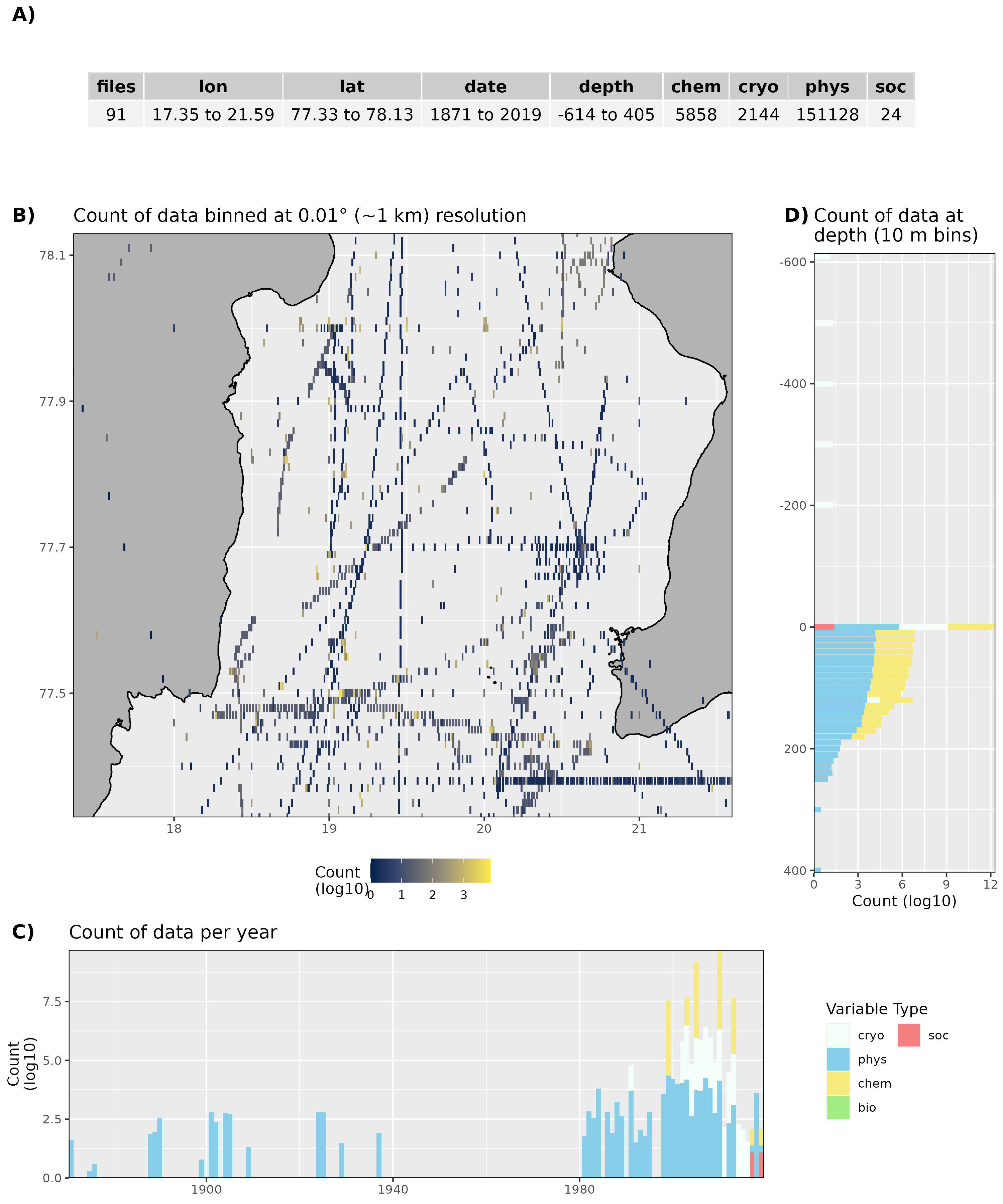
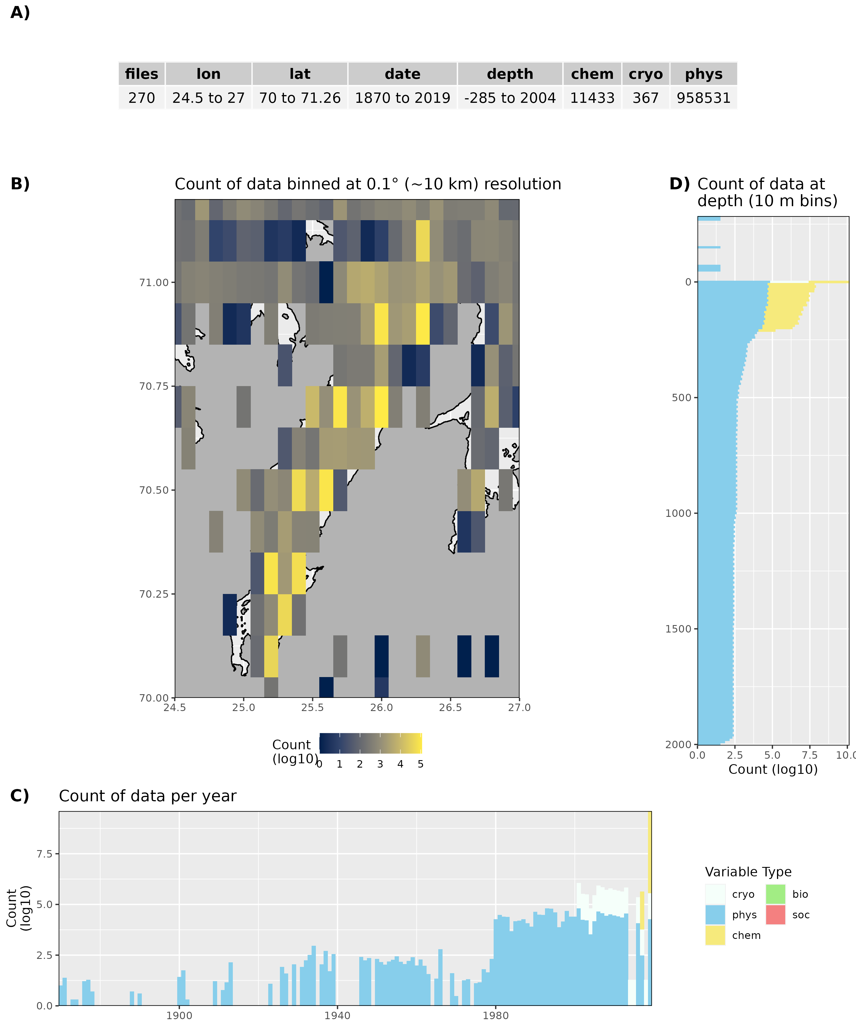
High level summary of data available for Kongsfjorden.
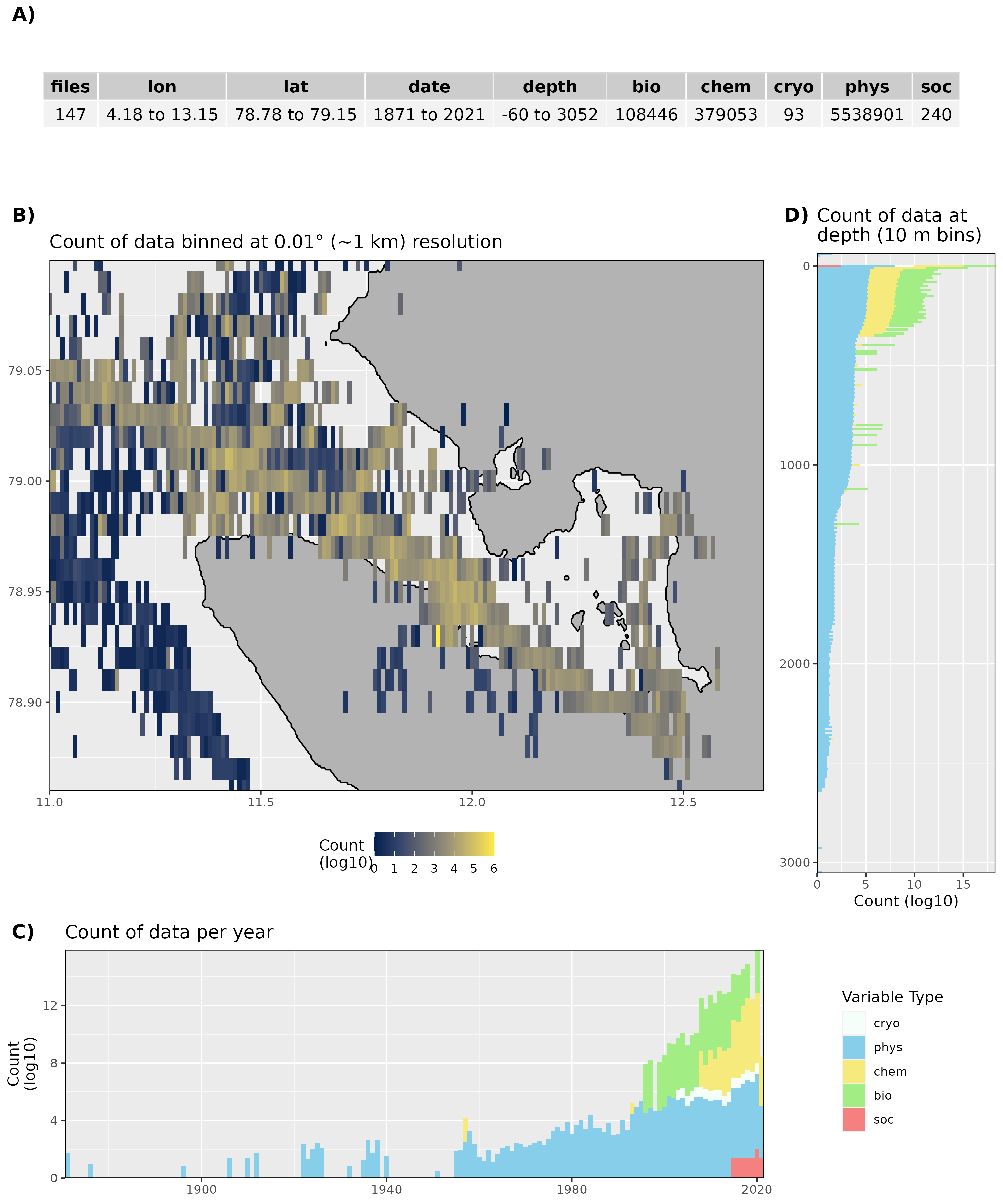
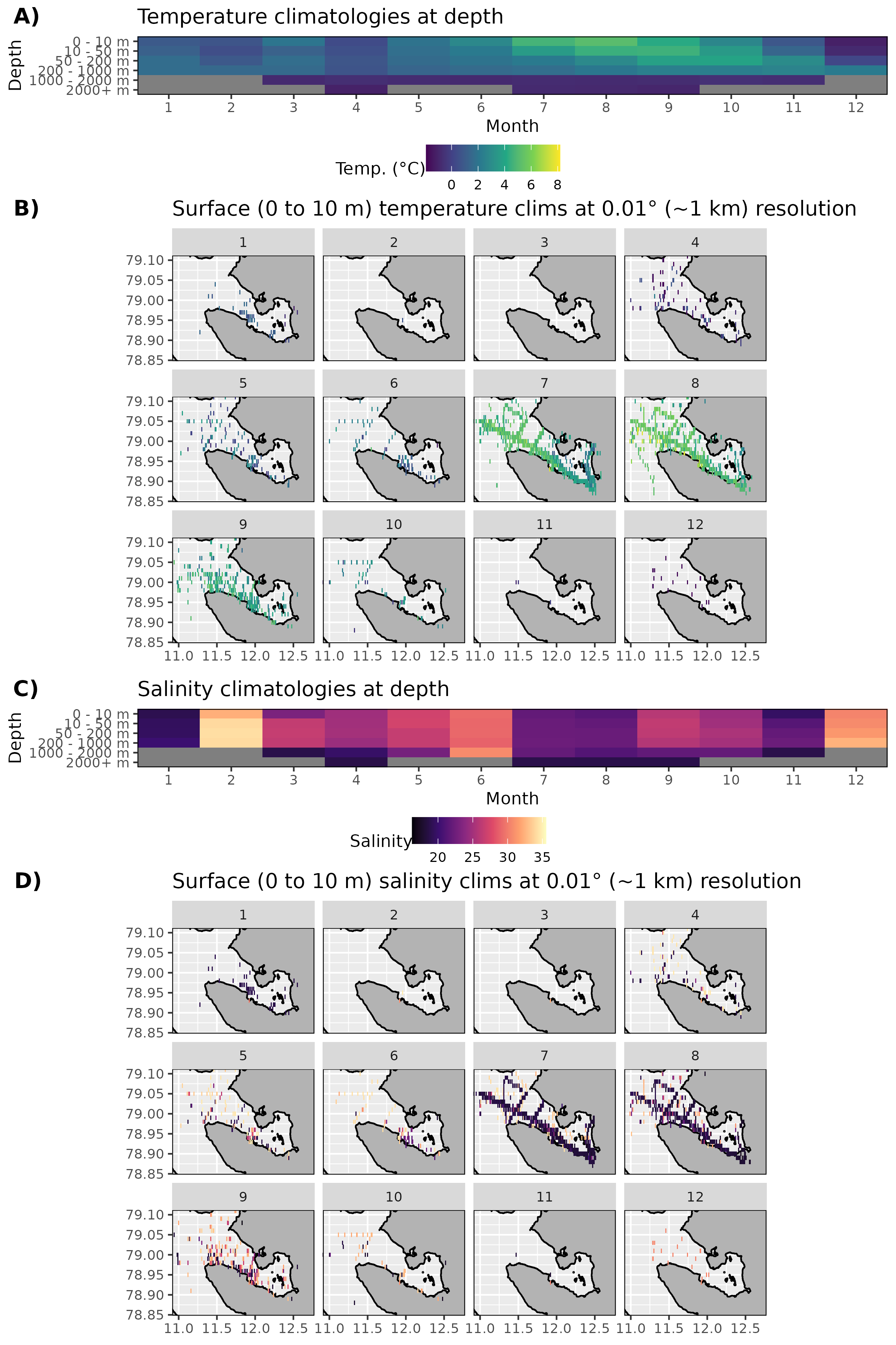
Monthly average values for temperature and salinity data. These are taken as illustrative figures for the data that are likely available per month as they are generally the two most highly sampled variables in marine science.
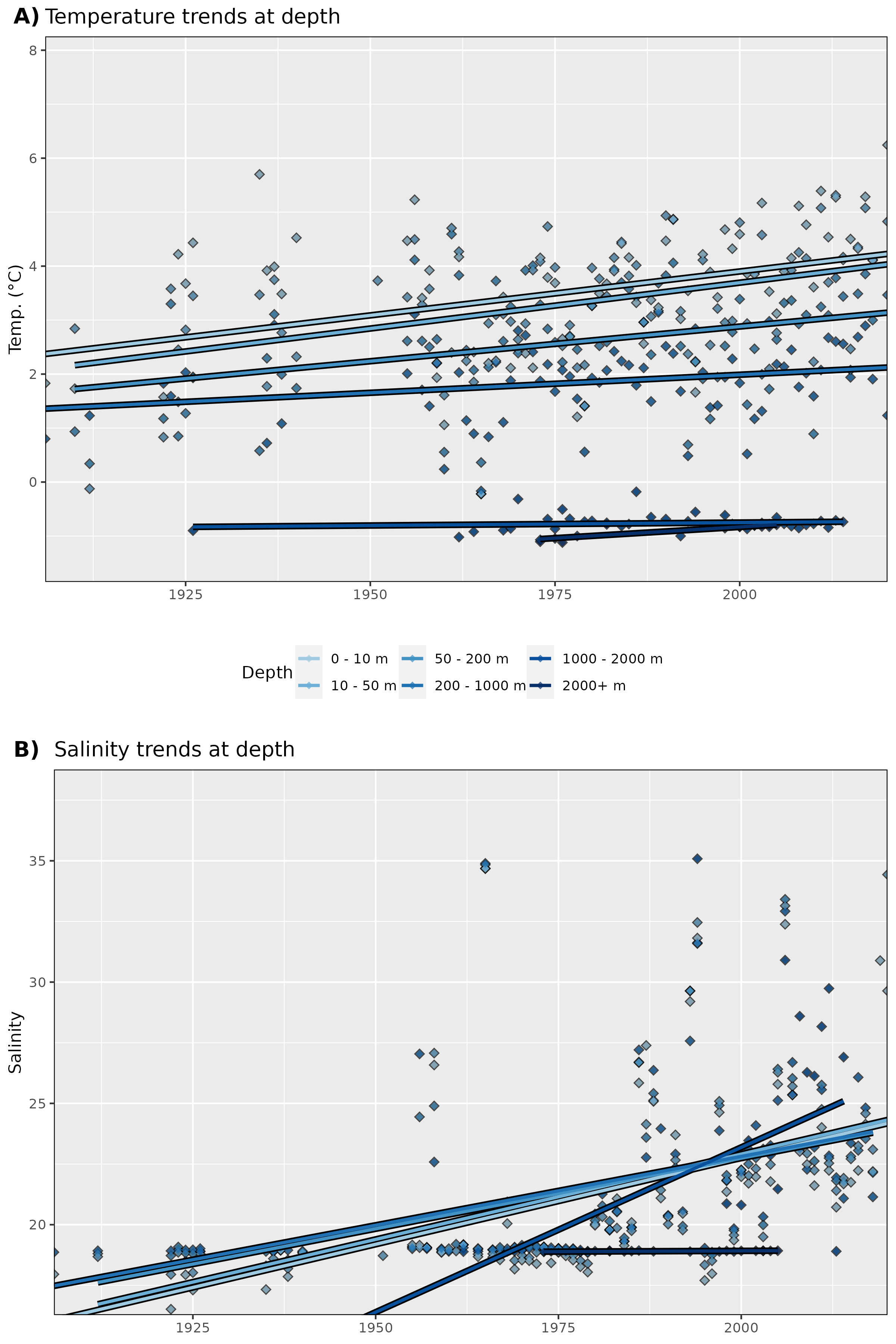
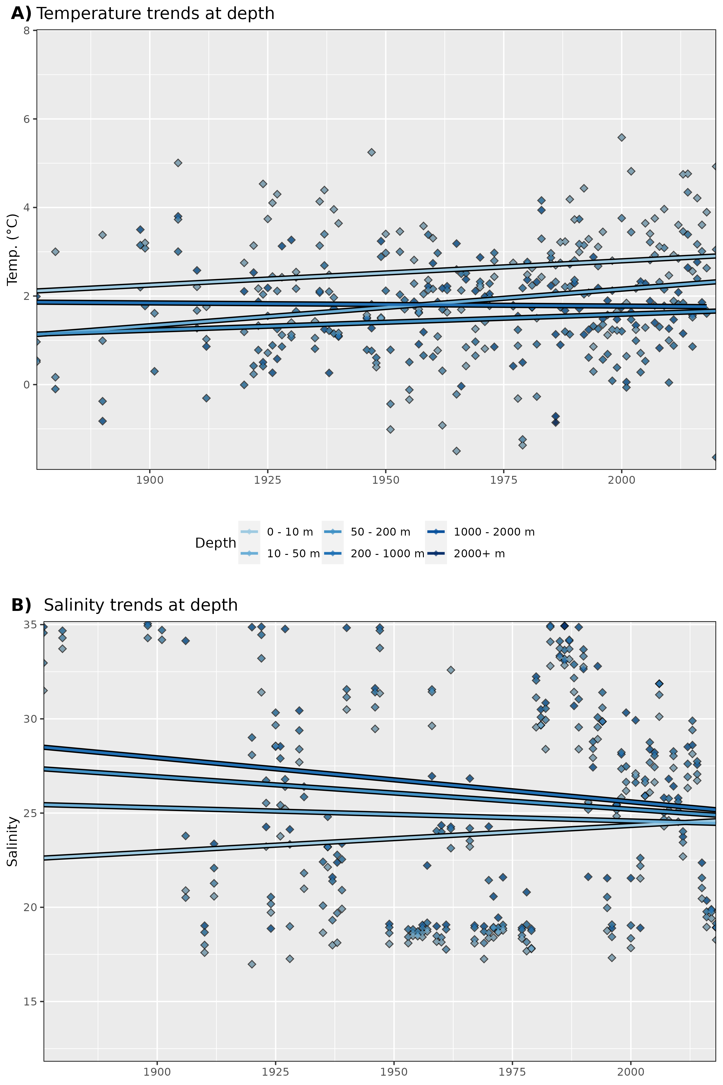
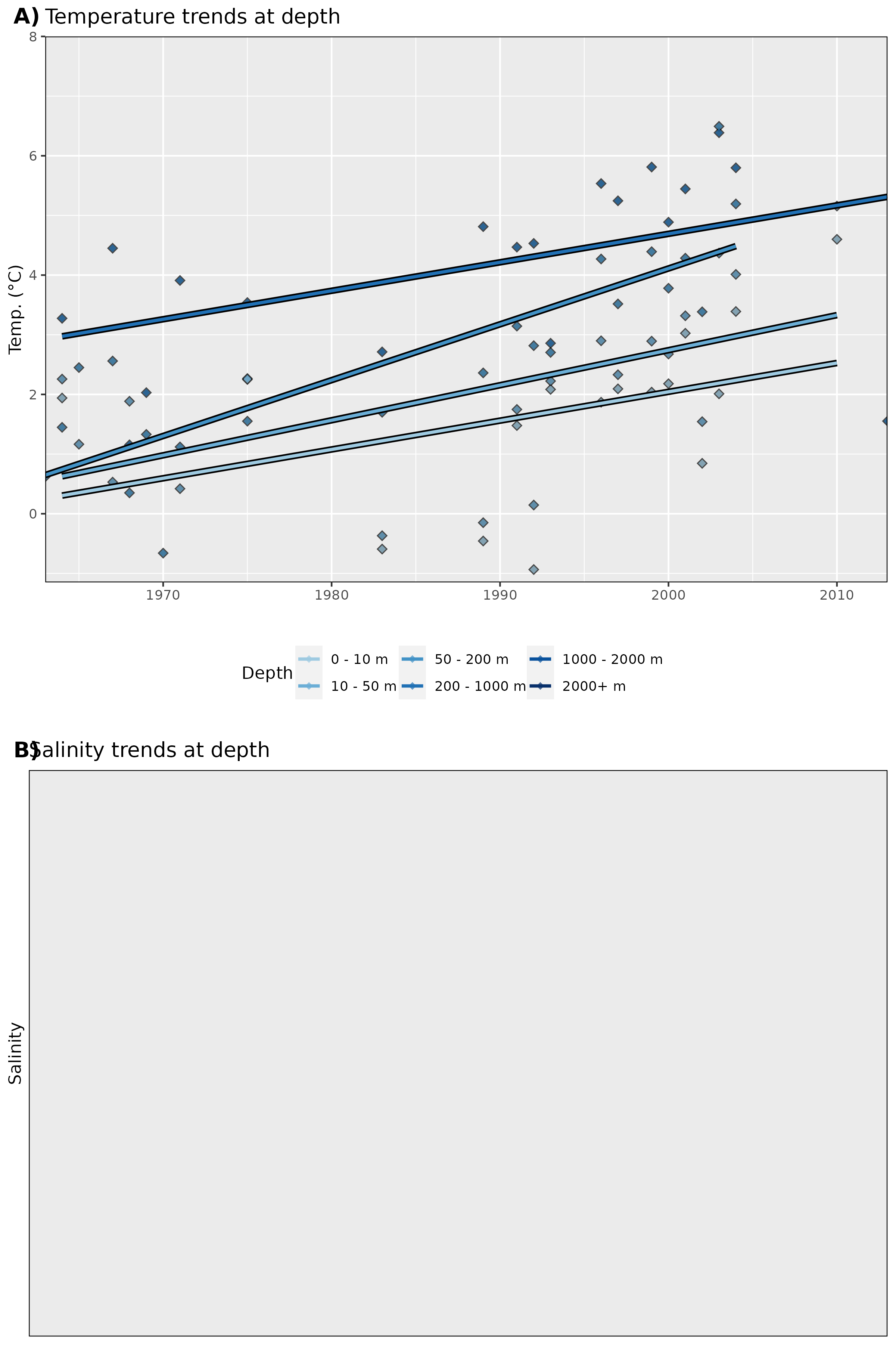
Trends in temperature and salinity data.
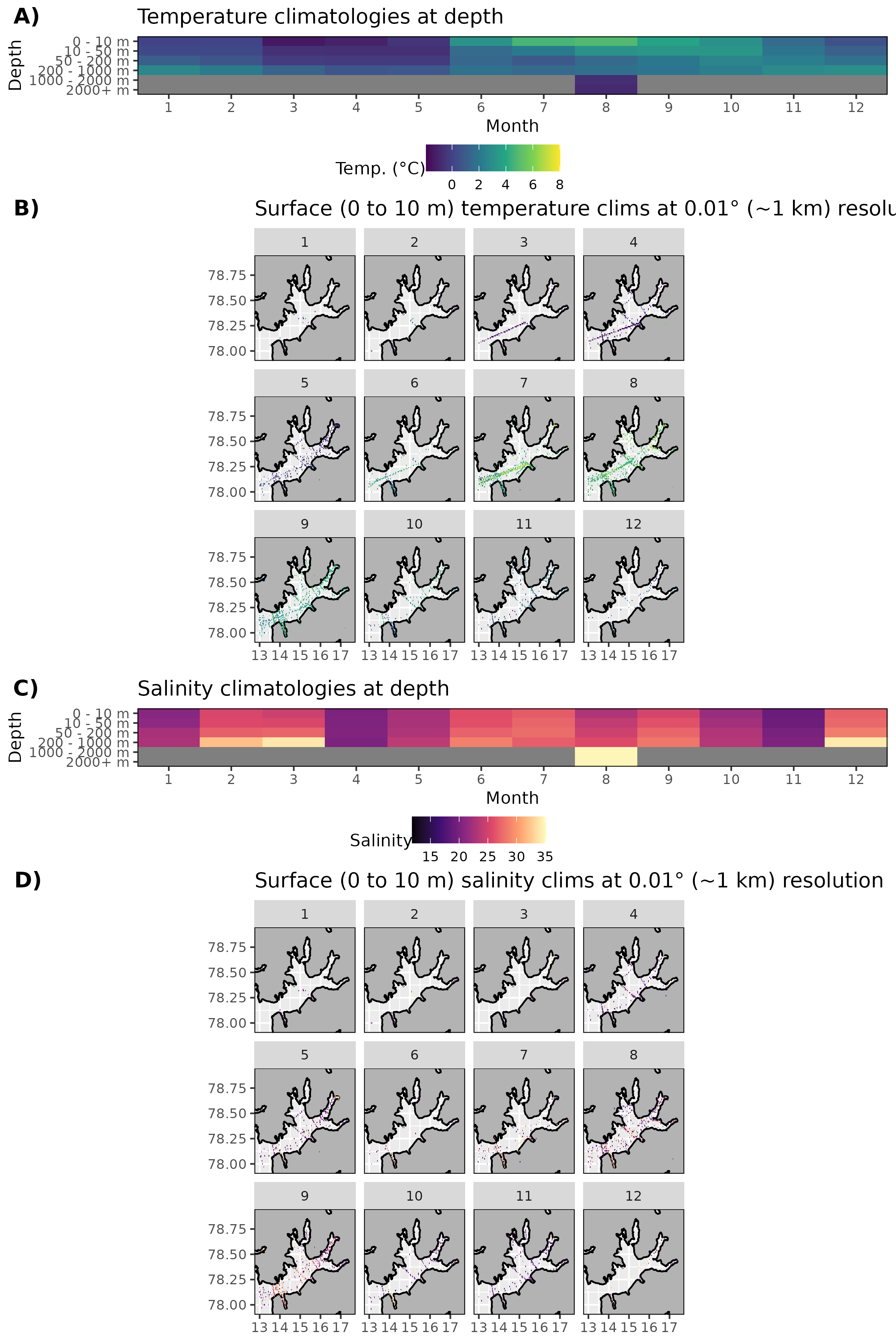
Isfjorden
High level summary of data available for Isfjorden.

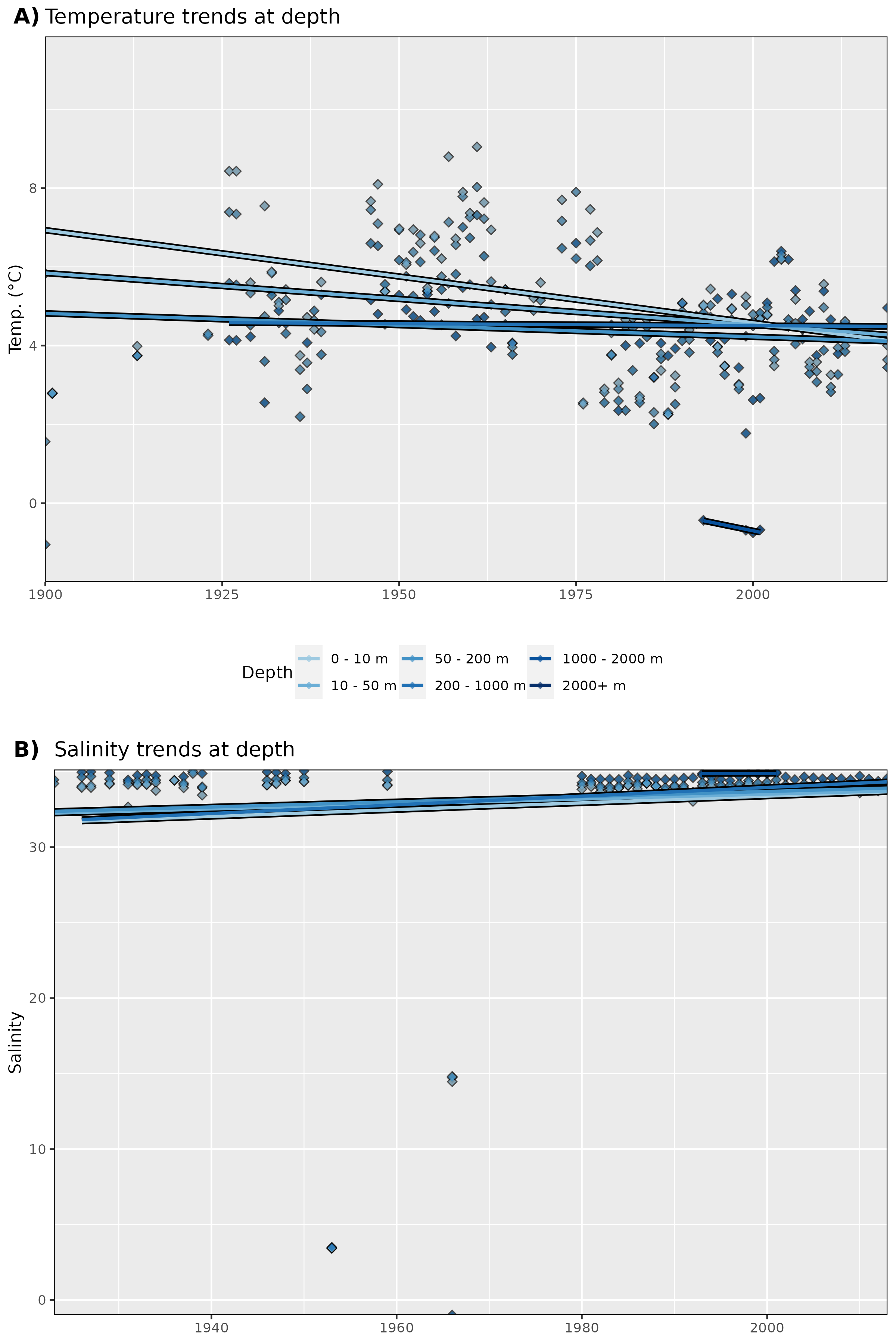
Monthly average values for temperature and salinity data.
Trends in temperature and salinity data.
Storfjorden
High level summary of data available for Storfjorden. This replaces the original site of Inglefieldbukta.
Monthly average values for temperature and salinity data.
Trends in temperature and salinity data.
Greenland
Young Sound
High level summary of data available for Young Sound.
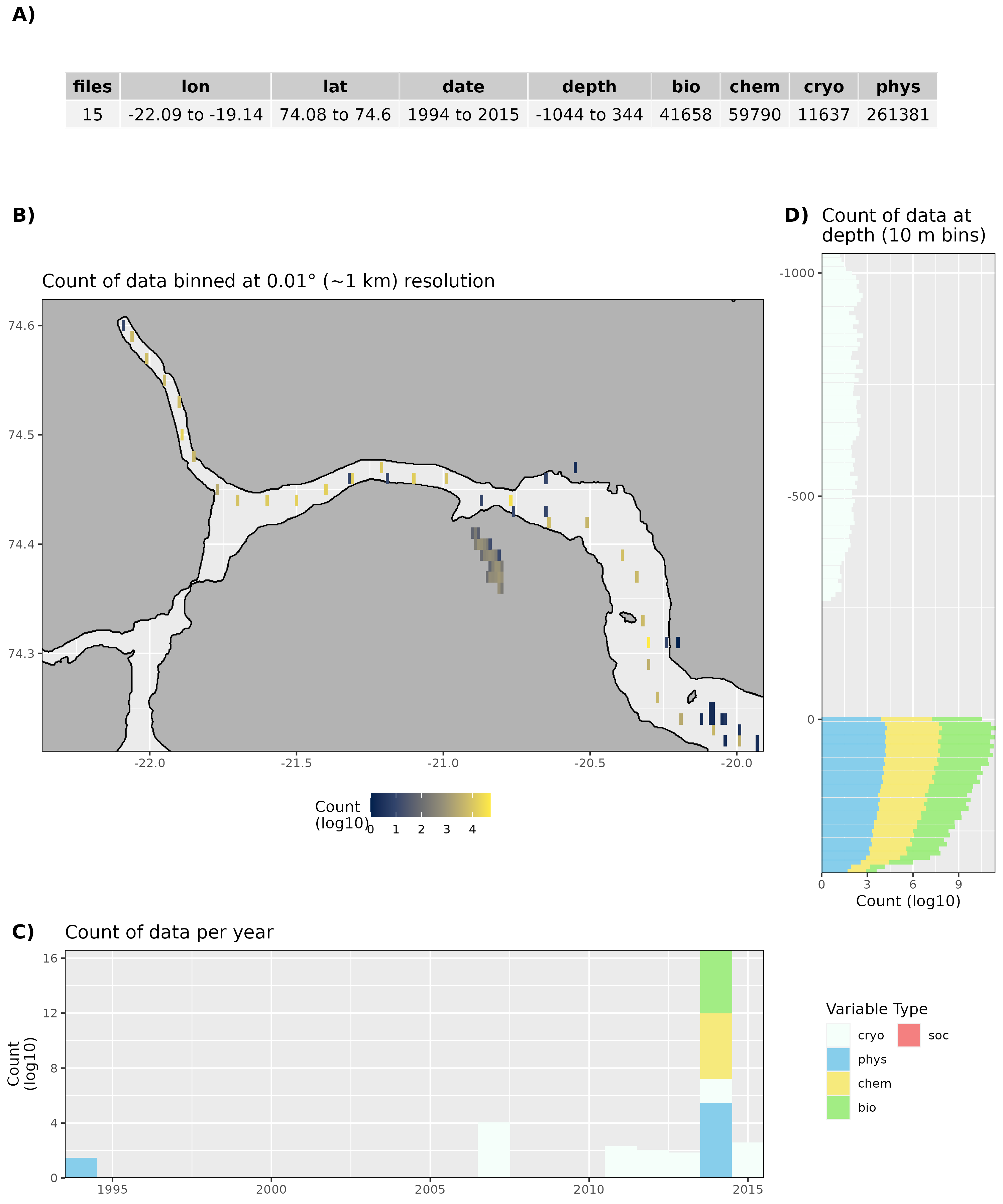
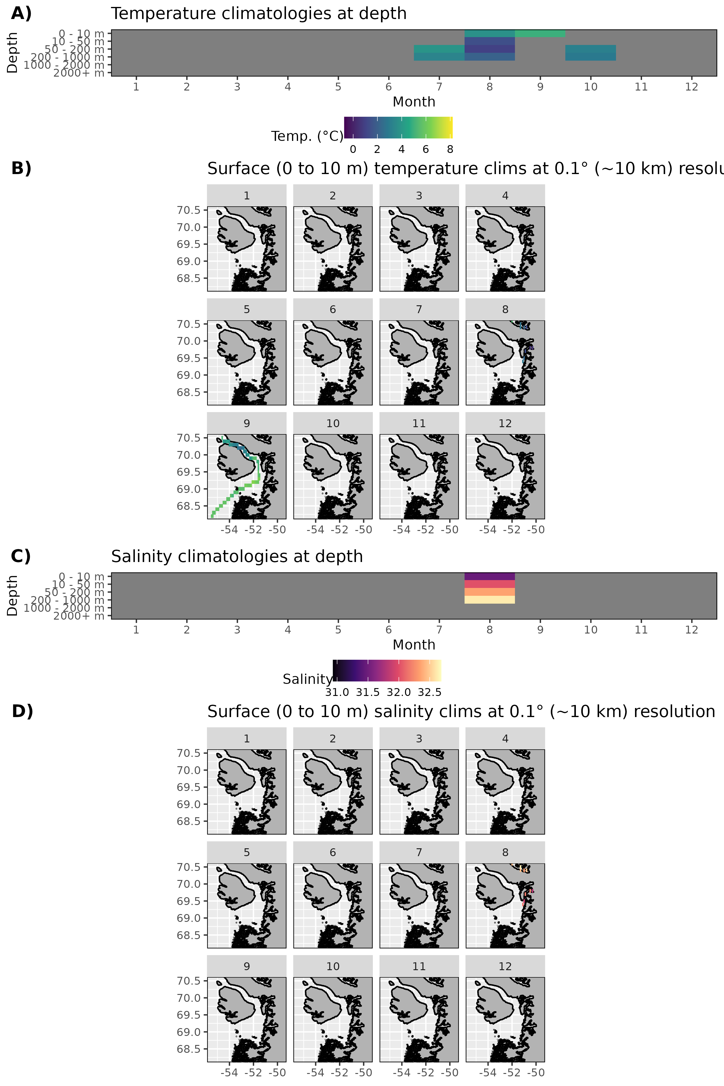
Monthly average values for temperature and salinity data.

Figure 11: Not enough data exist to calculate trends.
| Version | Author | Date |
|---|---|---|
| 7ad8a78 | Robert William Schlegel | 2023-12-12 |
| 610ff35 | Robert | 2023-08-30 |
| 6ad5b79 | Robert William Schlegel | 2023-08-24 |
| bd4819b | Robert | 2023-08-23 |
| 4ddbb12 | robwschlegel | 2023-07-24 |
| 2ea419c | Robert | 2023-05-30 |
| f59b5f2 | robwschlegel | 2022-11-28 |
| cc87bdd | Robert | 2022-09-23 |
| 8a8fd0b | Robert | 2022-05-27 |
| b32f47e | robwschlegel | 2022-04-21 |
| 0d6d433 | Robert | 2021-12-15 |
| cf10066 | robwschlegel | 2021-12-15 |
| 860f5d3 | Robert | 2021-12-10 |
| 2725466 | Robert | 2021-12-10 |
| 807675e | robwschlegel | 2021-12-06 |
| 104acbc | Robert | 2021-12-03 |
| 1e379a2 | robwschlegel | 2021-11-25 |
| b4d9162 | Robert | 2021-08-25 |
Trends in temperature and salinity data.

Figure 12: Not enough data exist to calculate trends.
| Version | Author | Date |
|---|---|---|
| 7ad8a78 | Robert William Schlegel | 2023-12-12 |
| 610ff35 | Robert | 2023-08-30 |
| 6ad5b79 | Robert William Schlegel | 2023-08-24 |
| bd4819b | Robert | 2023-08-23 |
| 4ddbb12 | robwschlegel | 2023-07-24 |
| 2ea419c | Robert | 2023-05-30 |
| f59b5f2 | robwschlegel | 2022-11-28 |
| cc87bdd | Robert | 2022-09-23 |
| 8a8fd0b | Robert | 2022-05-27 |
| b32f47e | robwschlegel | 2022-04-21 |
| 0d6d433 | Robert | 2021-12-15 |
| cf10066 | robwschlegel | 2021-12-15 |
| 860f5d3 | Robert | 2021-12-10 |
| 2725466 | Robert | 2021-12-10 |
| 807675e | robwschlegel | 2021-12-06 |
| 104acbc | Robert | 2021-12-03 |
| 1e379a2 | robwschlegel | 2021-11-25 |
| b4d9162 | Robert | 2021-08-25 |
Disko Bay
High level summary of data available for Disko Bay.
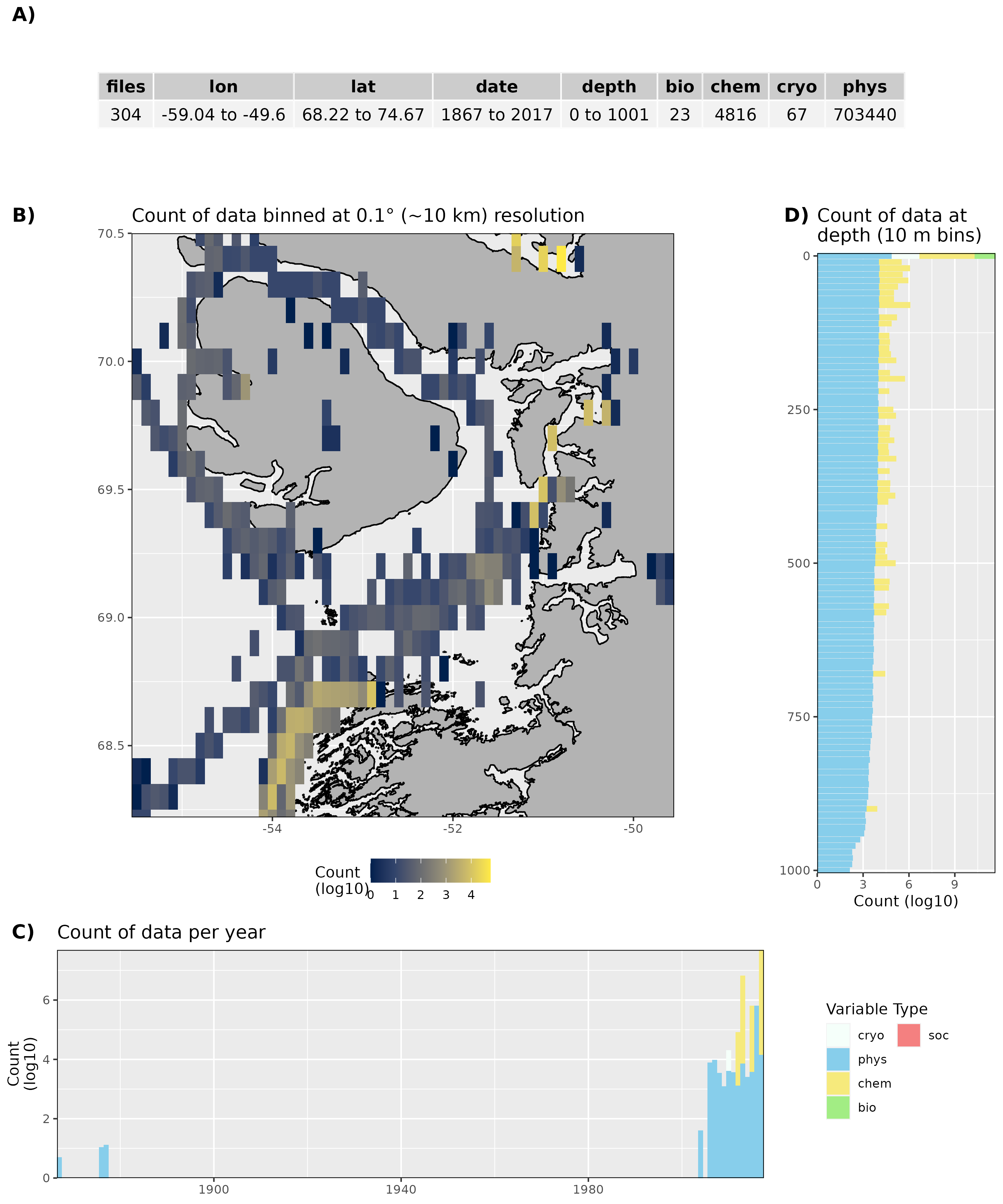
Monthly average values for temperature and salinity data.

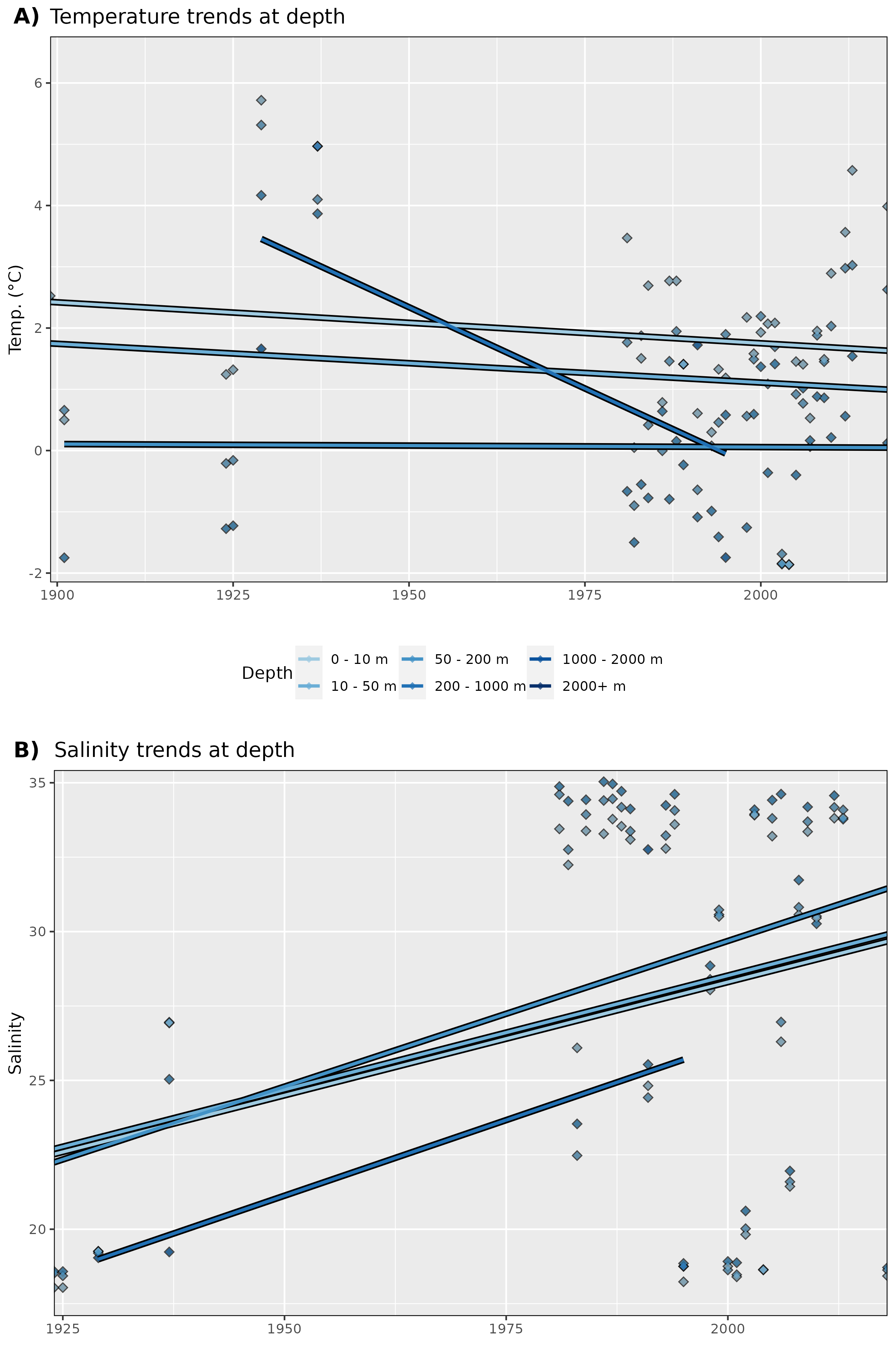
Trends in temperature and salinity data.

Figure 15: Not enough data exist to calculate trends.
| Version | Author | Date |
|---|---|---|
| 7ad8a78 | Robert William Schlegel | 2023-12-12 |
| 610ff35 | Robert | 2023-08-30 |
| 6ad5b79 | Robert William Schlegel | 2023-08-24 |
| bd4819b | Robert | 2023-08-23 |
| 4ddbb12 | robwschlegel | 2023-07-24 |
| 2ea419c | Robert | 2023-05-30 |
| f59b5f2 | robwschlegel | 2022-11-28 |
| cc87bdd | Robert | 2022-09-23 |
| 8a8fd0b | Robert | 2022-05-27 |
| b32f47e | robwschlegel | 2022-04-21 |
| 0d6d433 | Robert | 2021-12-15 |
| cf10066 | robwschlegel | 2021-12-15 |
| 860f5d3 | Robert | 2021-12-10 |
| 2725466 | Robert | 2021-12-10 |
| 807675e | robwschlegel | 2021-12-06 |
| 104acbc | Robert | 2021-12-03 |
| 1e379a2 | robwschlegel | 2021-11-25 |
| b4d9162 | Robert | 2021-08-25 |
Nuup Kangerlua
High level summary of data available for Nuup Kangerlua.
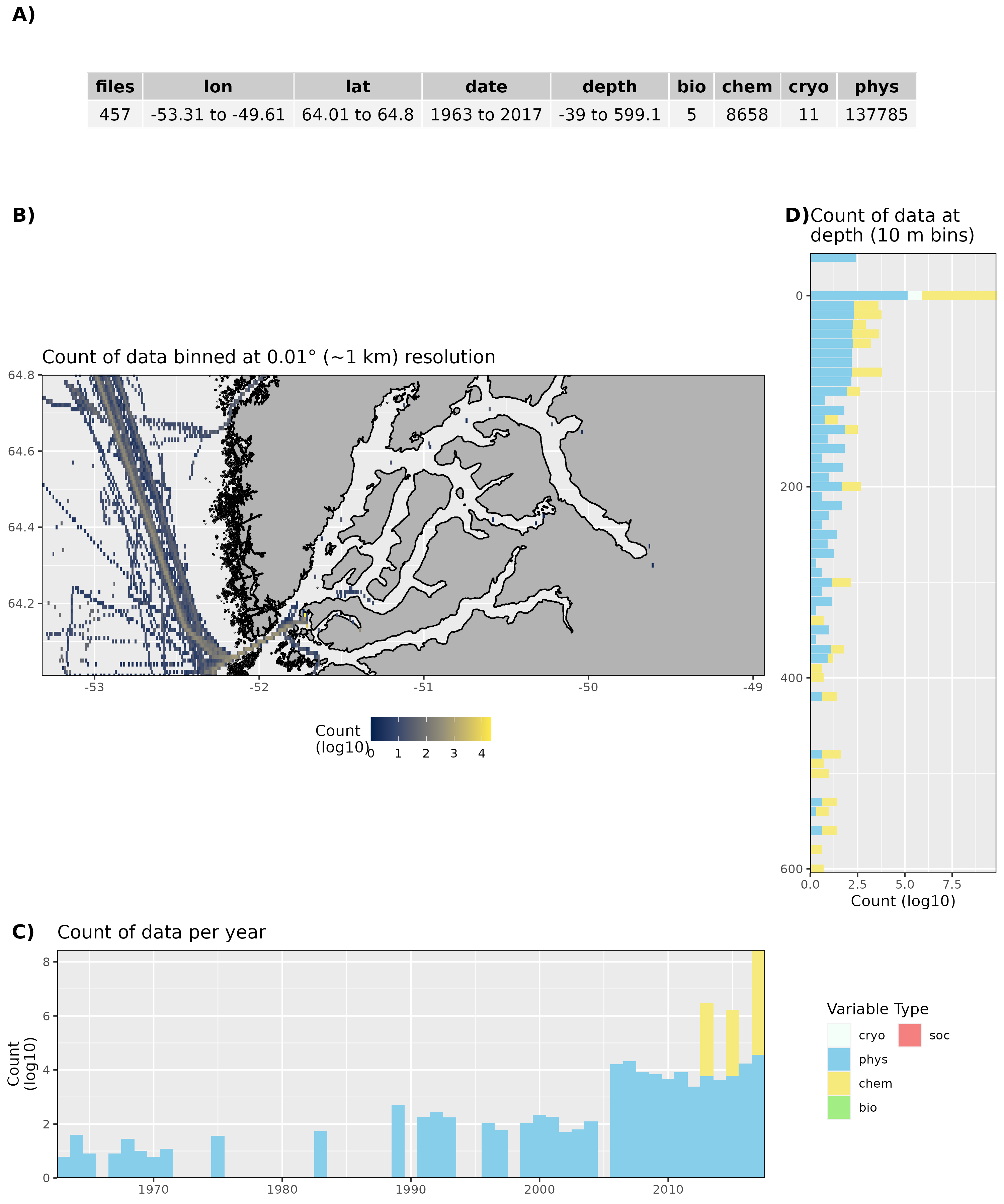
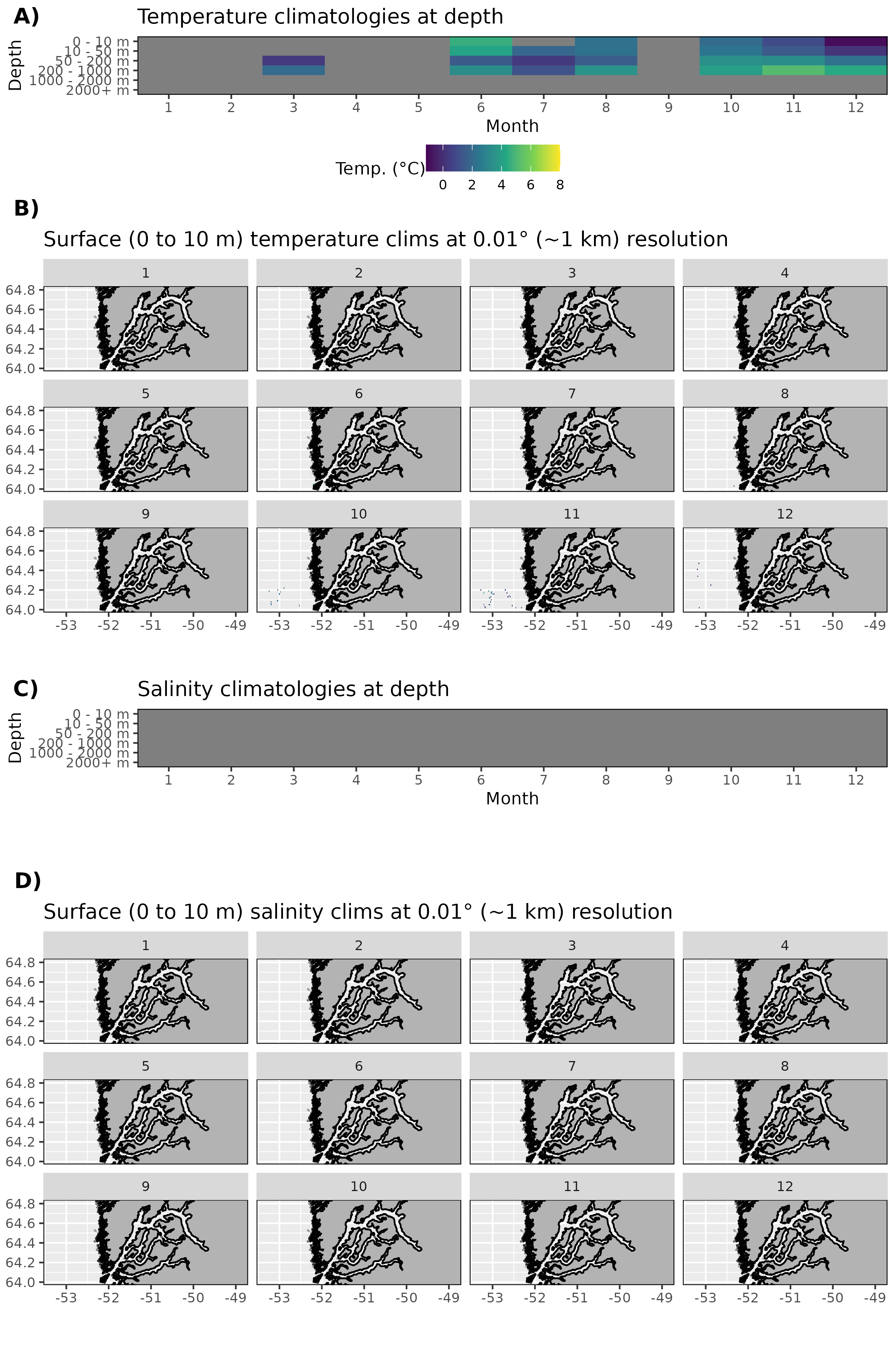
Monthly average values for temperature and salinity data.
Trends in temperature and salinity data.
Norway
Porsangerfjorden
High level summary of data available for Porsangerfjorden.
Monthly average values for temperature and salinity data.

Trends in temperature and salinity data.
References
R version 4.4.1 (2024-06-14)
Platform: x86_64-pc-linux-gnu
Running under: Ubuntu 22.04.5 LTS

Matrix products: default
BLAS:   /usr/lib/x86_64-linux-gnu/blas/libblas.so.3.10.0
LAPACK: /usr/lib/x86_64-linux-gnu/lapack/liblapack.so.3.10.0

locale:
 [1] LC_CTYPE=en_GB.UTF-8       LC_NUMERIC=C
 [3] LC_TIME=fr_FR.UTF-8        LC_COLLATE=en_GB.UTF-8
 [5] LC_MONETARY=fr_FR.UTF-8    LC_MESSAGES=en_GB.UTF-8
 [7] LC_PAPER=fr_FR.UTF-8       LC_NAME=C
 [9] LC_ADDRESS=C               LC_TELEPHONE=C
[11] LC_MEASUREMENT=fr_FR.UTF-8 LC_IDENTIFICATION=C

time zone: UTC
tzcode source: system (glibc)

attached base packages:
[1] stats     graphics  grDevices utils     datasets  methods   base

other attached packages:
 [1] lubridate_1.9.3 forcats_1.0.0   stringr_1.5.1   dplyr_1.1.4
 [5] purrr_1.0.2     readr_2.1.5     tidyr_1.3.1     tibble_3.2.1
 [9] ggplot2_3.5.1   tidyverse_2.0.0 workflowr_1.7.1

loaded via a namespace (and not attached):
 [1] sass_0.4.9        utf8_1.2.4        generics_0.1.3    stringi_1.8.4
 [5] hms_1.1.3         digest_0.6.37     magrittr_2.0.3    timechange_0.3.0
 [9] evaluate_0.24.0   grid_4.4.1        fastmap_1.2.0     rprojroot_2.0.4
[13] jsonlite_1.8.8    processx_3.8.4    whisker_0.4.1     ps_1.8.0
[17] promises_1.3.0    httr_1.4.7        fansi_1.0.6       scales_1.3.0
[21] jquerylib_0.1.4   cli_3.6.3         rlang_1.1.4       munsell_0.5.1
[25] withr_3.0.1       cachem_1.1.0      yaml_2.3.10       tools_4.4.1
[29] tzdb_0.4.0        colorspace_2.1-1  httpuv_1.6.15     vctrs_0.6.5
[33] R6_2.5.1          lifecycle_1.0.4   git2r_0.33.0      fs_1.6.4
[37] pkgconfig_2.0.3   callr_3.7.6       pillar_1.9.0      bslib_0.8.0
[41] later_1.3.2       gtable_0.3.5      glue_1.7.0        Rcpp_1.0.13
[45] highr_0.11        xfun_0.47         tidyselect_1.2.1  rstudioapi_0.16.0
[49] knitr_1.48        farver_2.1.2      htmltools_0.5.8.1 labeling_0.4.3
[53] rmarkdown_2.28    compiler_4.4.1    getPass_0.2-4