Last updated: 2024-03-20

Checks: 7 0

Knit directory: WP1/

This reproducible R Markdown analysis was created with workflowr (version 1.7.1). The Checks tab describes the reproducibility checks that were applied when the results were created. The Past versions tab lists the development history.


Great! Since the R Markdown file has been committed to the Git repository, you know the exact version of the code that produced these results.

Great job! The global environment was empty. Objects defined in the global environment can affect the analysis in your R Markdown file in unknown ways. For reproduciblity it’s best to always run the code in an empty environment.

The command set.seed(20210216) was run prior to running the code in the R Markdown file. Setting a seed ensures that any results that rely on randomness, e.g. subsampling or permutations, are reproducible.

Great job! Recording the operating system, R version, and package versions is critical for reproducibility.

Nice! There were no cached chunks for this analysis, so you can be confident that you successfully produced the results during this run.

Great job! Using relative paths to the files within your workflowr project makes it easier to run your code on other machines.

Great! You are using Git for version control. Tracking code development and connecting the code version to the results is critical for reproducibility.

The results in this page were generated with repository version 2492e14. See the Past versions tab to see a history of the changes made to the R Markdown and HTML files.

Note that you need to be careful to ensure that all relevant files for the analysis have been committed to Git prior to generating the results (you can use wflow_publish or wflow_git_commit). workflowr only checks the R Markdown file, but you know if there are other scripts or data files that it depends on. Below is the status of the Git repository when the results were generated:


Ignored files:
    Ignored:    .Rhistory
    Ignored:    .Rproj.user/
    Ignored:    .httr-oauth
    Ignored:    code/.Rhistory
    Ignored:    data/analyses/clean_all.RData
    Ignored:    data/analyses/clean_all_clean.RData
    Ignored:    data/analyses/ice_4km_proc.RData
    Ignored:    data/full_data/
    Ignored:    data/sst_trom.RData
    Ignored:    metadata/globalfishingwatch_API_key.RData
    Ignored:    metadata/is_gfw_database.RData
    Ignored:    metadata/pangaea_parameters.tab
    Ignored:    metadata/pg_EU_ref_meta.csv
    Ignored:    mhw-definition_1_orig.xcf
    Ignored:    poster/SSC_2021_landscape_files/paged-0.15/
    Ignored:    presentations/.Rhistory
    Ignored:    presentations/2023_Ilico.html
    Ignored:    presentations/2023_LOV.html
    Ignored:    presentations/2023_results_day.html
    Ignored:    presentations/2023_seminar.html
    Ignored:    presentations/2023_summary.html
    Ignored:    presentations/2024_36_month.html
    Ignored:    presentations/2024_seminar.html
    Ignored:    presentations/ASSW_2023.html
    Ignored:    presentations/ASSW_side_2023.html
    Ignored:    presentations/Session5_SCHLEGEL.html
    Ignored:    shiny/dataAccess/coastline_hi_sub.csv
    Ignored:    shiny/kongCTD/.httr-oauth
    Ignored:    shiny/kongCTD/credentials.RData
    Ignored:    shiny/kongCTD/data/
    Ignored:    shiny/test_data/

Unstaged changes:
    Modified:   analysis/_site.yml

Note that any generated files, e.g. HTML, png, CSS, etc., are not included in this status report because it is ok for generated content to have uncommitted changes.


These are the previous versions of the repository in which changes were made to the R Markdown (analysis/sst_summary.Rmd) and HTML (docs/sst_summary.html) files. If you’ve configured a remote Git repository (see ?wflow_git_remote), click on the hyperlinks in the table below to view the files as they were in that past version.

File Version Author Date Message
html 2bba2c0 Robert William Schlegel 2024-01-25 Build site.
html 9228f25 Robert William Schlegel 2023-12-20 Build site.
html 0926ac4 Robert William Schlegel 2023-12-12 Build site.
html 7ad8a78 Robert William Schlegel 2023-12-12 Build site.
html 77b2a61 Robert 2023-12-04 Build site.
html 610ff35 Robert 2023-08-30 Build site.
html 6ad5b79 Robert William Schlegel 2023-08-24 Build site.
html bd4819b Robert 2023-08-23 Build site.
html 4ddbb12 robwschlegel 2023-07-24 Build site.
html e8997de Robert 2023-05-30 Build site.
html 2ea419c Robert 2023-05-30 Build site.
html f59b5f2 robwschlegel 2022-11-28 Re-published site
html cc87bdd Robert 2022-09-23 Build site.
html 8a8fd0b Robert 2022-05-27 Build site.
html b32f47e robwschlegel 2022-04-21 Build site.
html 1d3a3b3 Robert 2021-12-17 Build site.
html 122fbe4 Robert 2021-12-17 New Young Sound data
html 0d6d433 Robert 2021-12-15 Build site.
html cf10066 robwschlegel 2021-12-15 Build site.
Rmd dd7b8a0 robwschlegel 2021-12-15 Re-built site.
html dd7b8a0 robwschlegel 2021-12-15 Re-built site.
html 4cdbd33 robwschlegel 2021-12-15 Build site.
Rmd 993272c robwschlegel 2021-12-15 Re-built site.
html 5ba8046 Robert 2021-12-15 Build site.
Rmd bc740fa Robert 2021-12-15 Added a bit of text
html bc740fa Robert 2021-12-15 Added a bit of text
html 57f4772 Robert 2021-12-15 Build site.
Rmd 713428c Robert 2021-12-15 Calculated SST trends for all model data
html 713428c Robert 2021-12-15 Calculated SST trends for all model data
html 1beea50 Robert 2021-12-14 Build site.
html b554c7a Robert 2021-12-14 Fixed labelling for CCI SST figures
html 1da6285 Robert 2021-12-14 Build site.
Rmd 1b3e2f2 Robert 2021-12-14 Added CCI SST analysis and figures to the SST data page
html 1b3e2f2 Robert 2021-12-14 Added CCI SST analysis and figures to the SST data page
html 860f5d3 Robert 2021-12-10 Build site.
html 2725466 Robert 2021-12-10 Merge
html 64a5252 Robert 2021-12-10 Build site.
html 807675e robwschlegel 2021-12-06 Build site.
html 104acbc Robert 2021-12-03 Build site.
Rmd e8e7420 Robert 2021-12-03 SST analysis figures
html e8e7420 Robert 2021-12-03 SST analysis figures

Overview

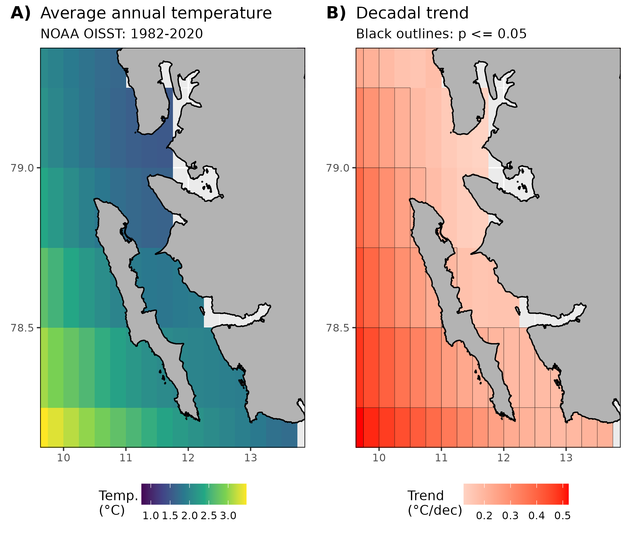
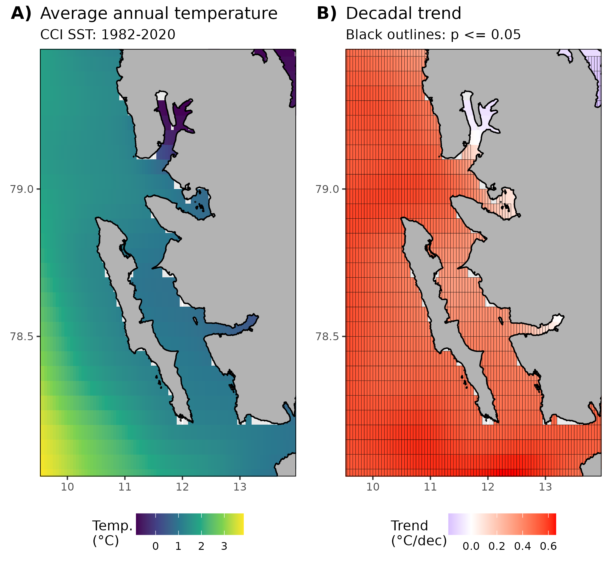
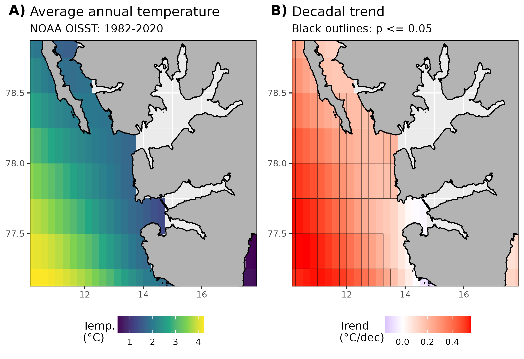
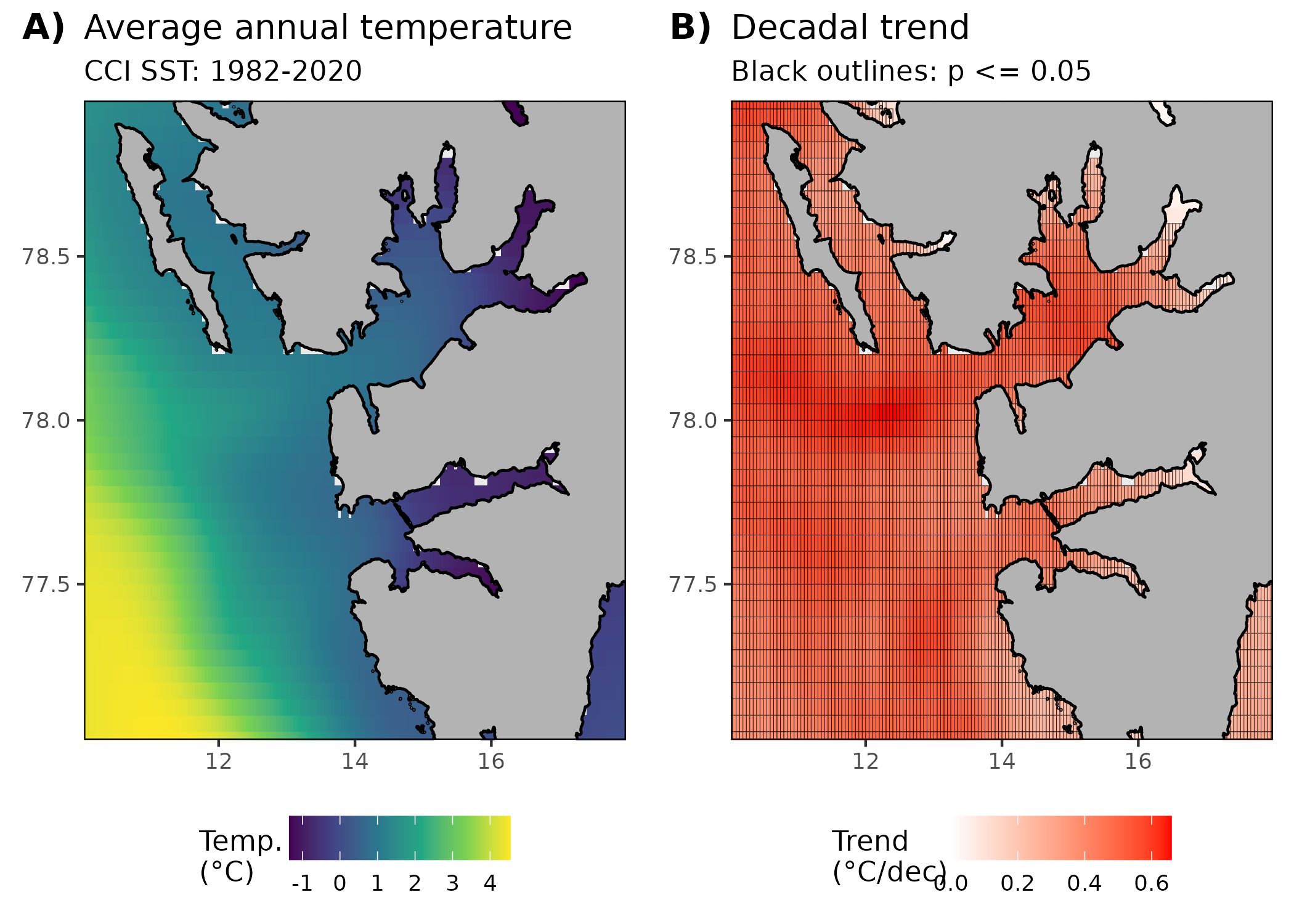
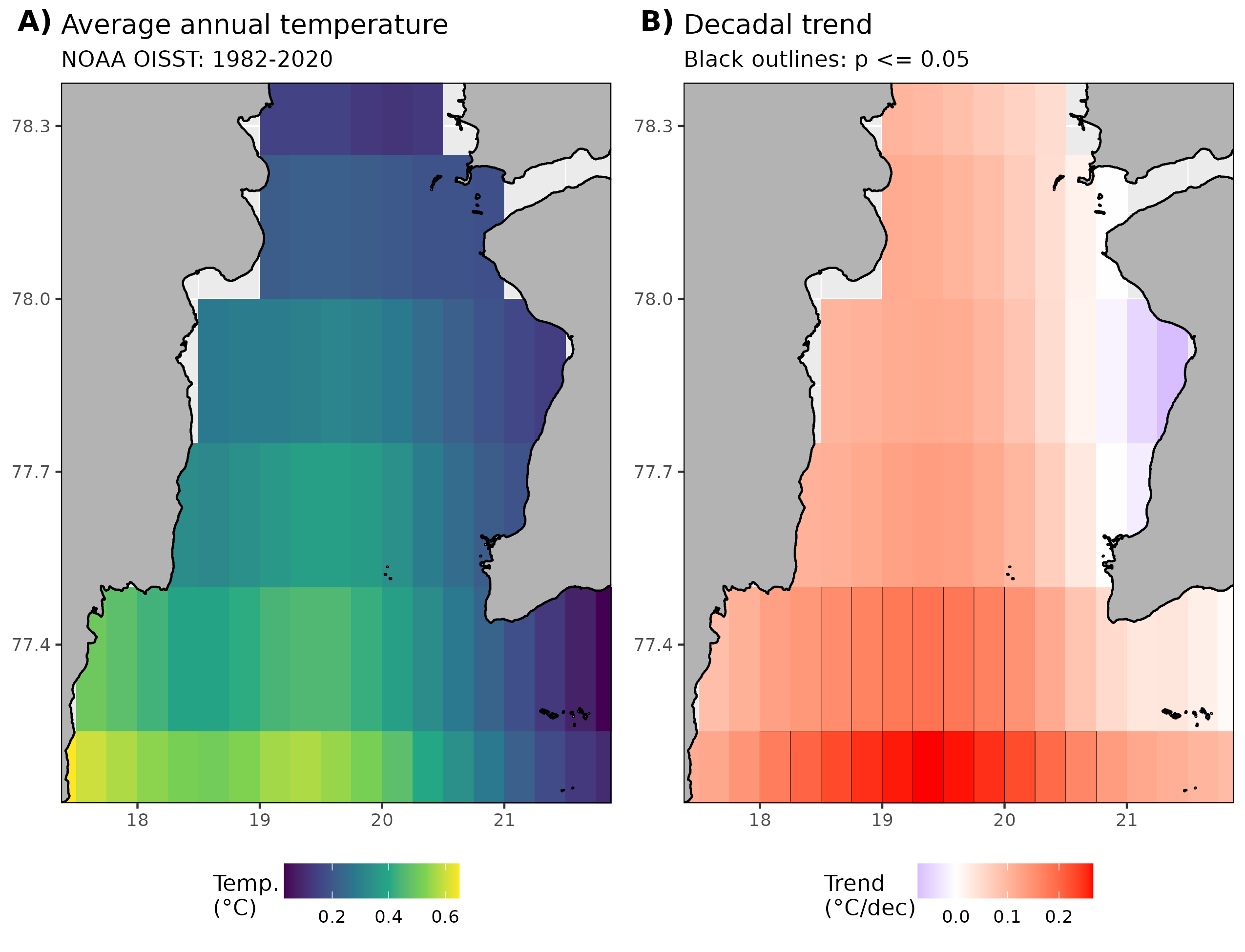
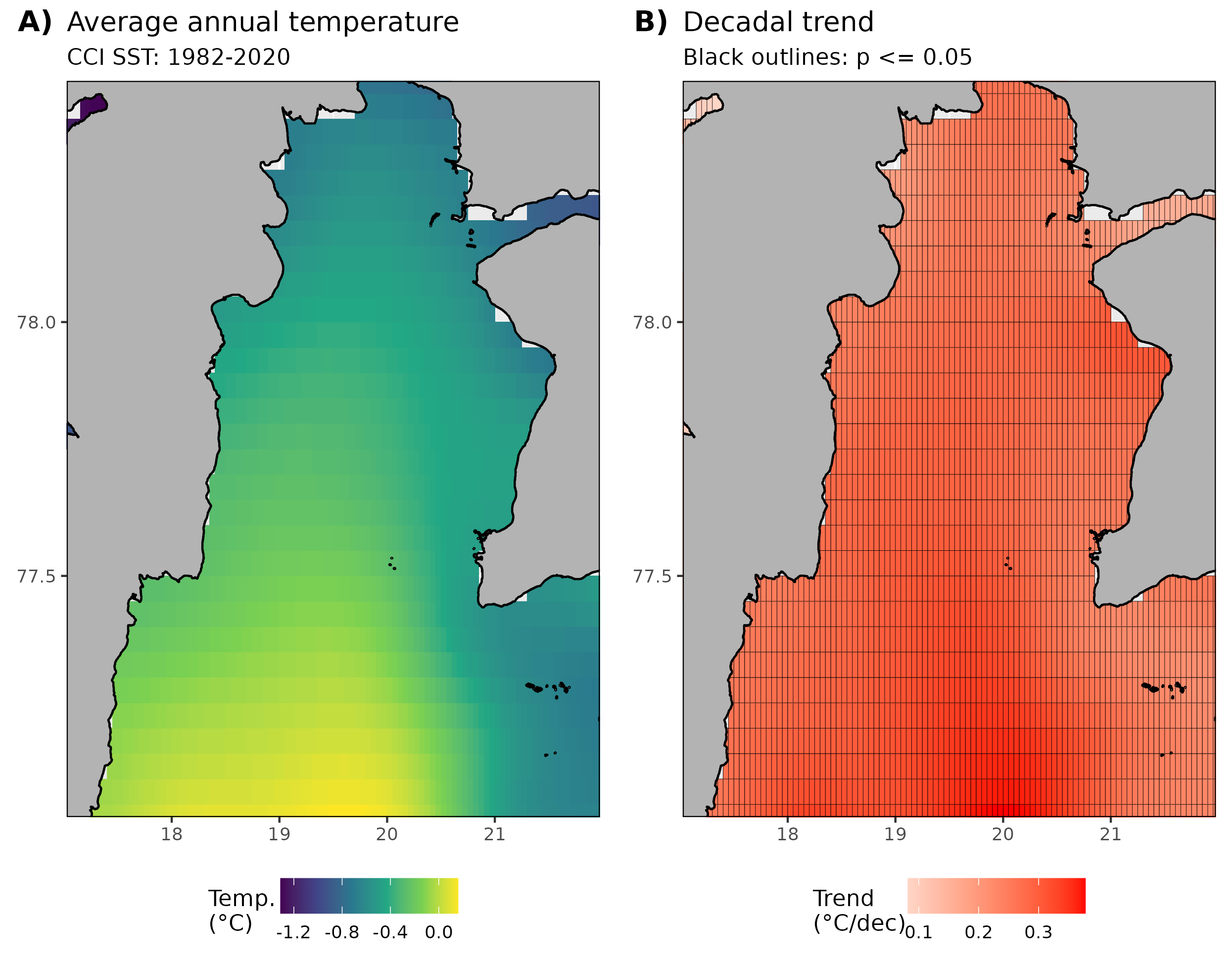
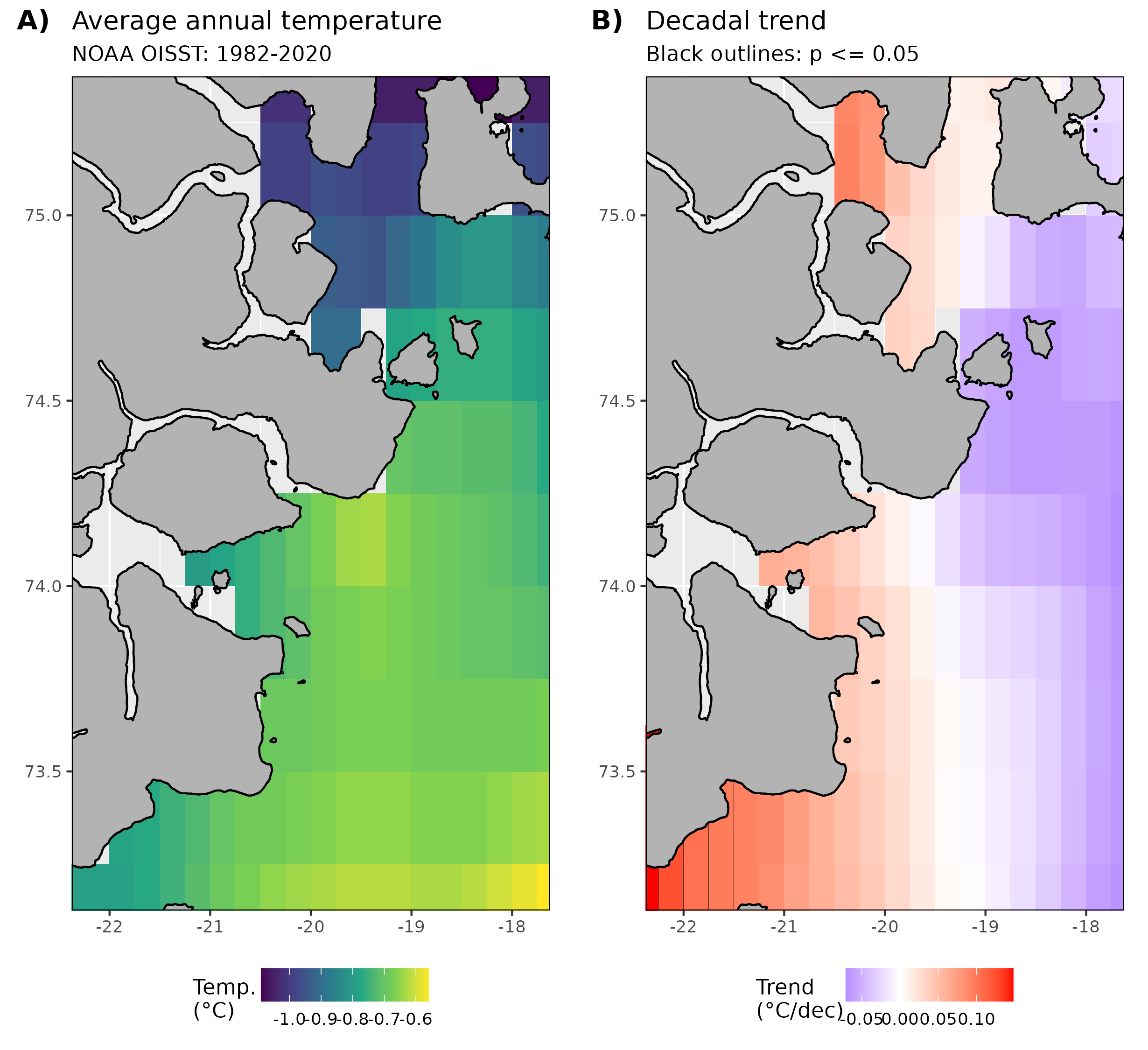
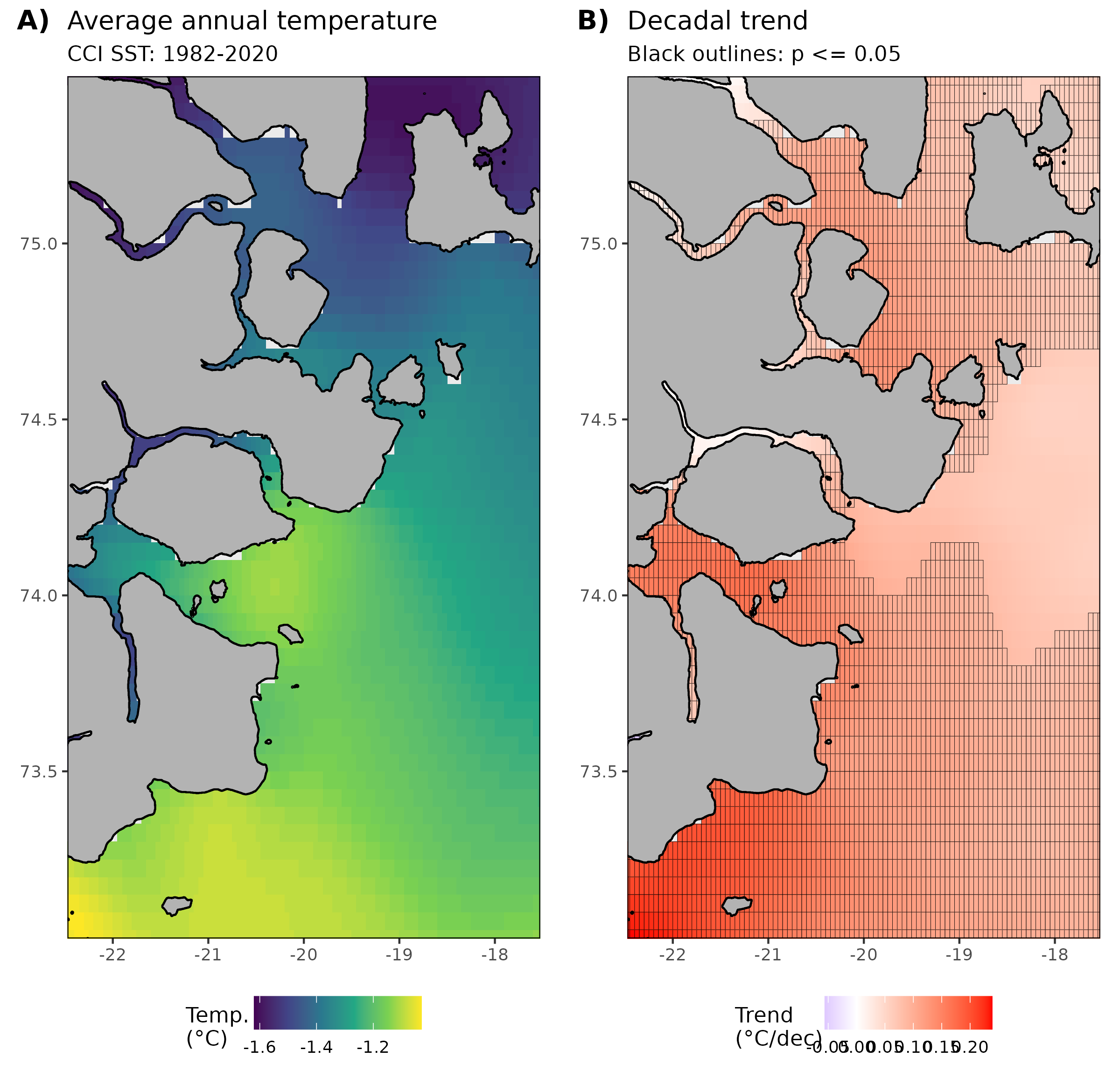
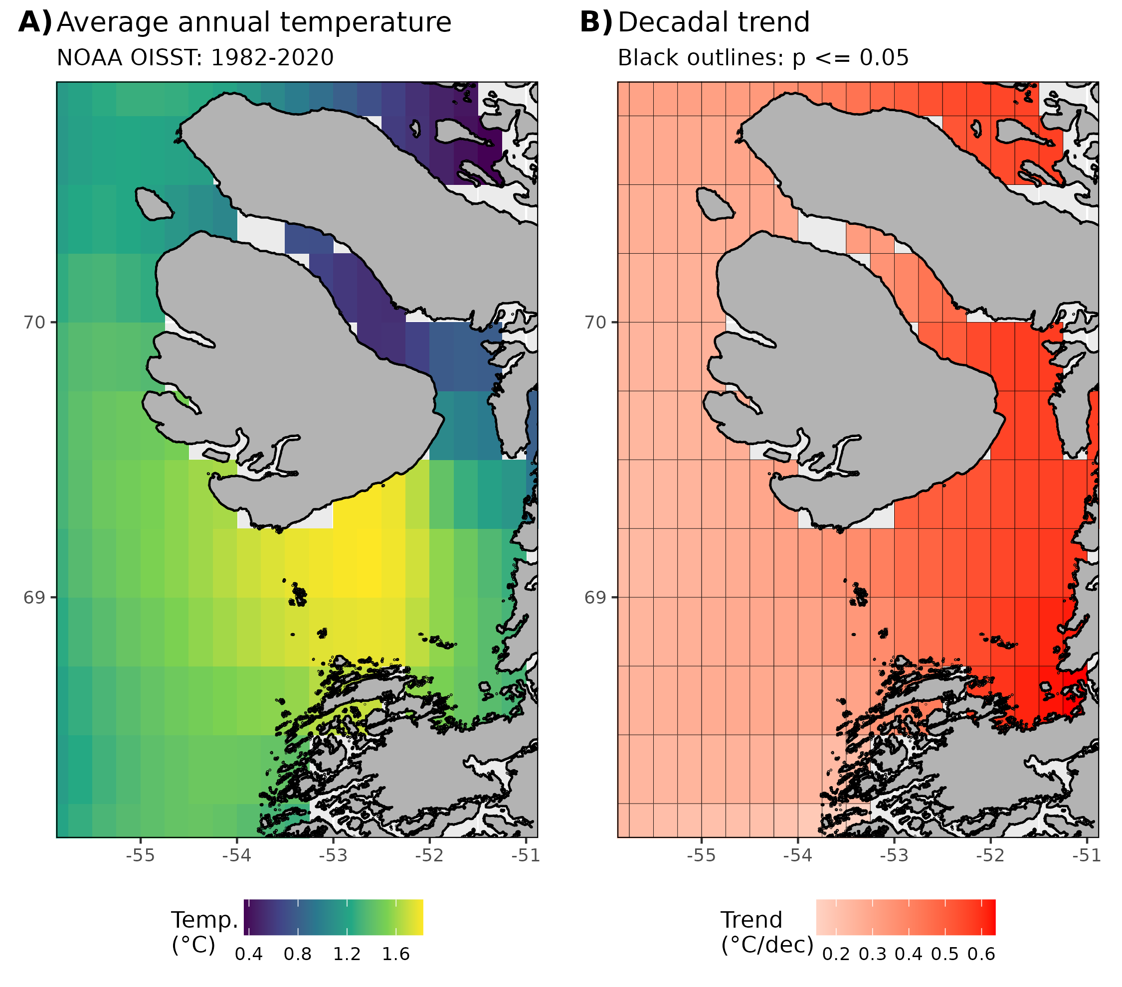
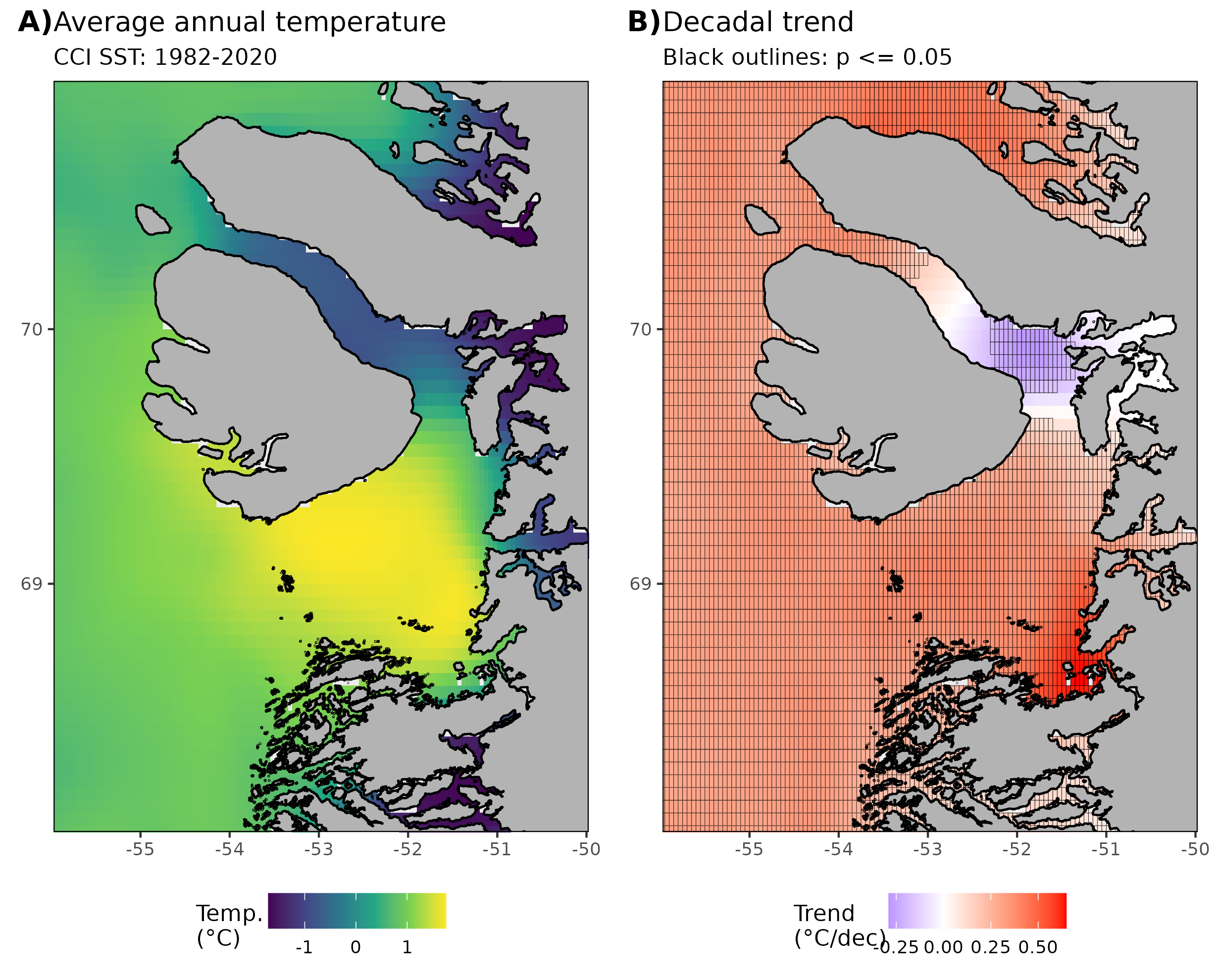
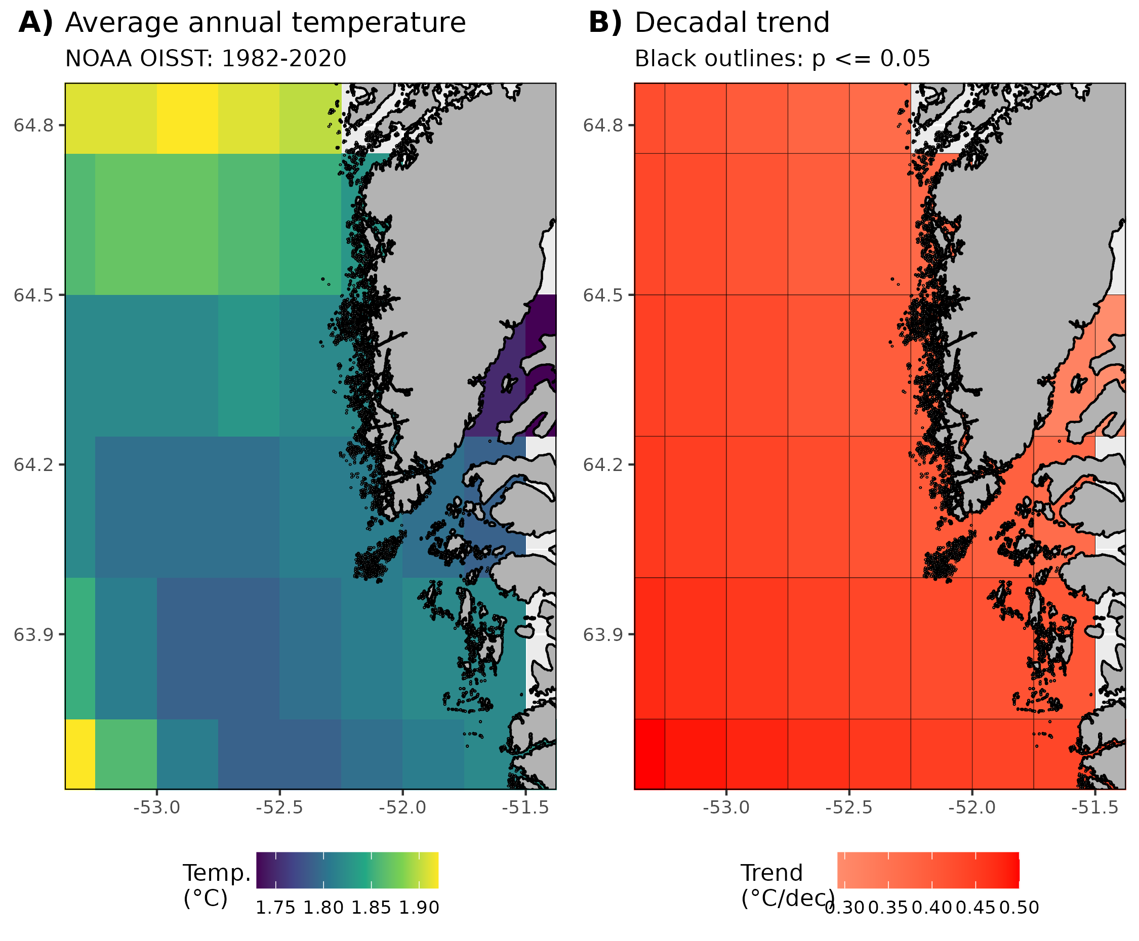
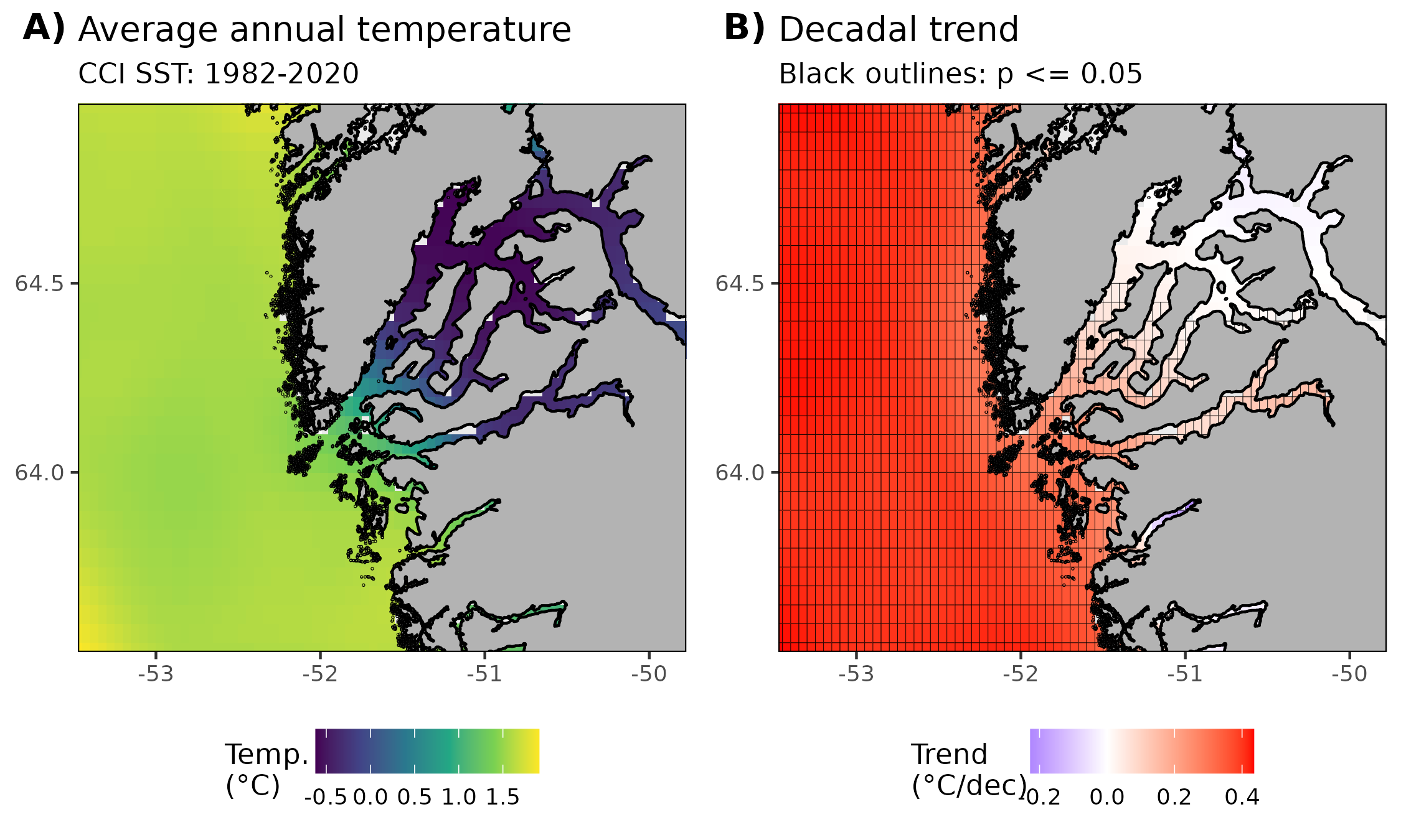
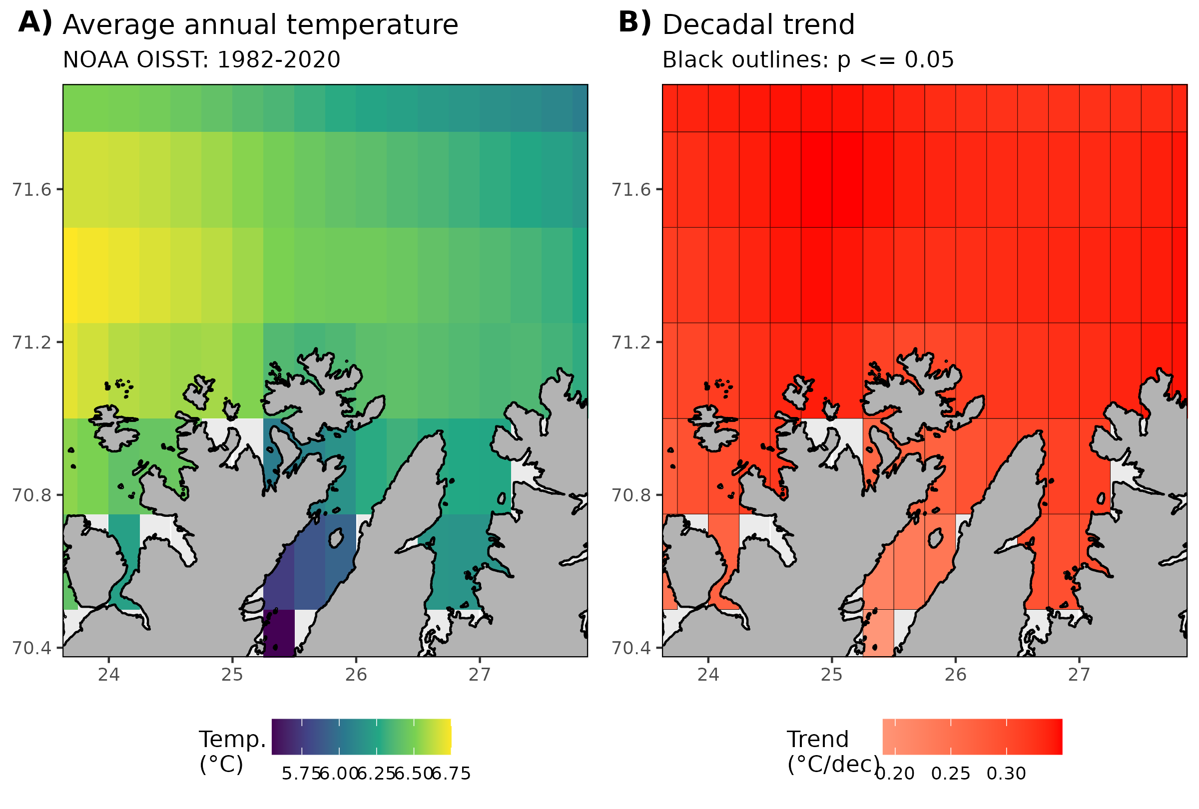
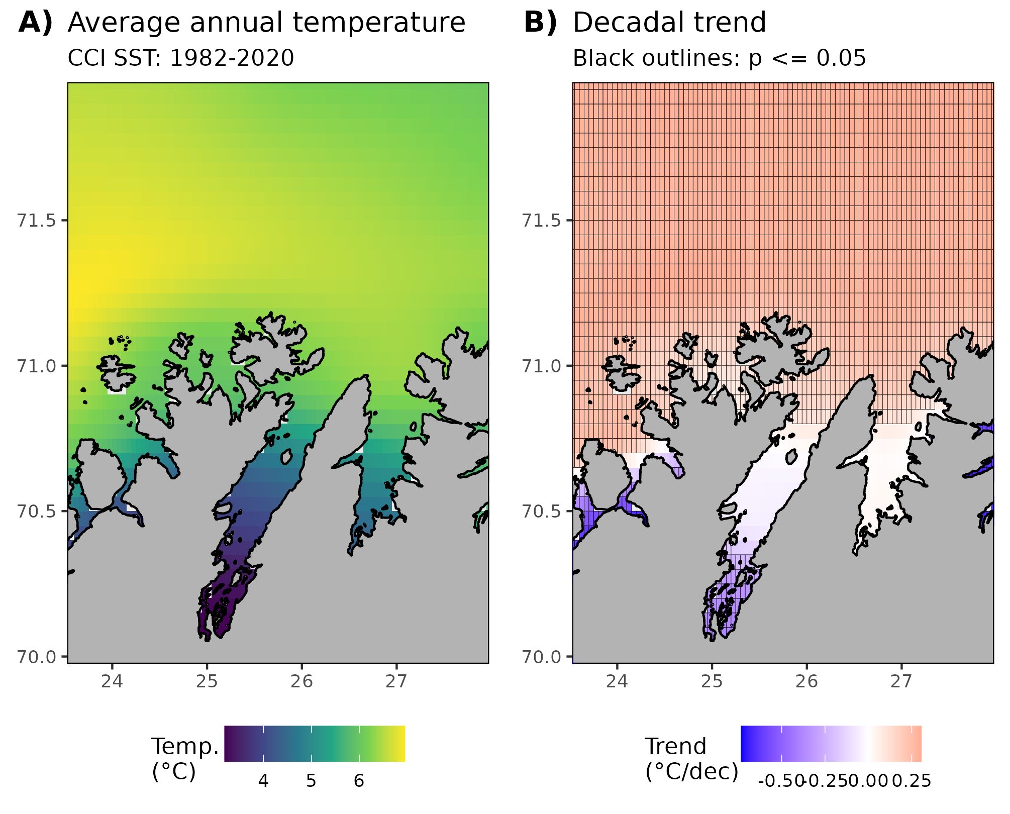
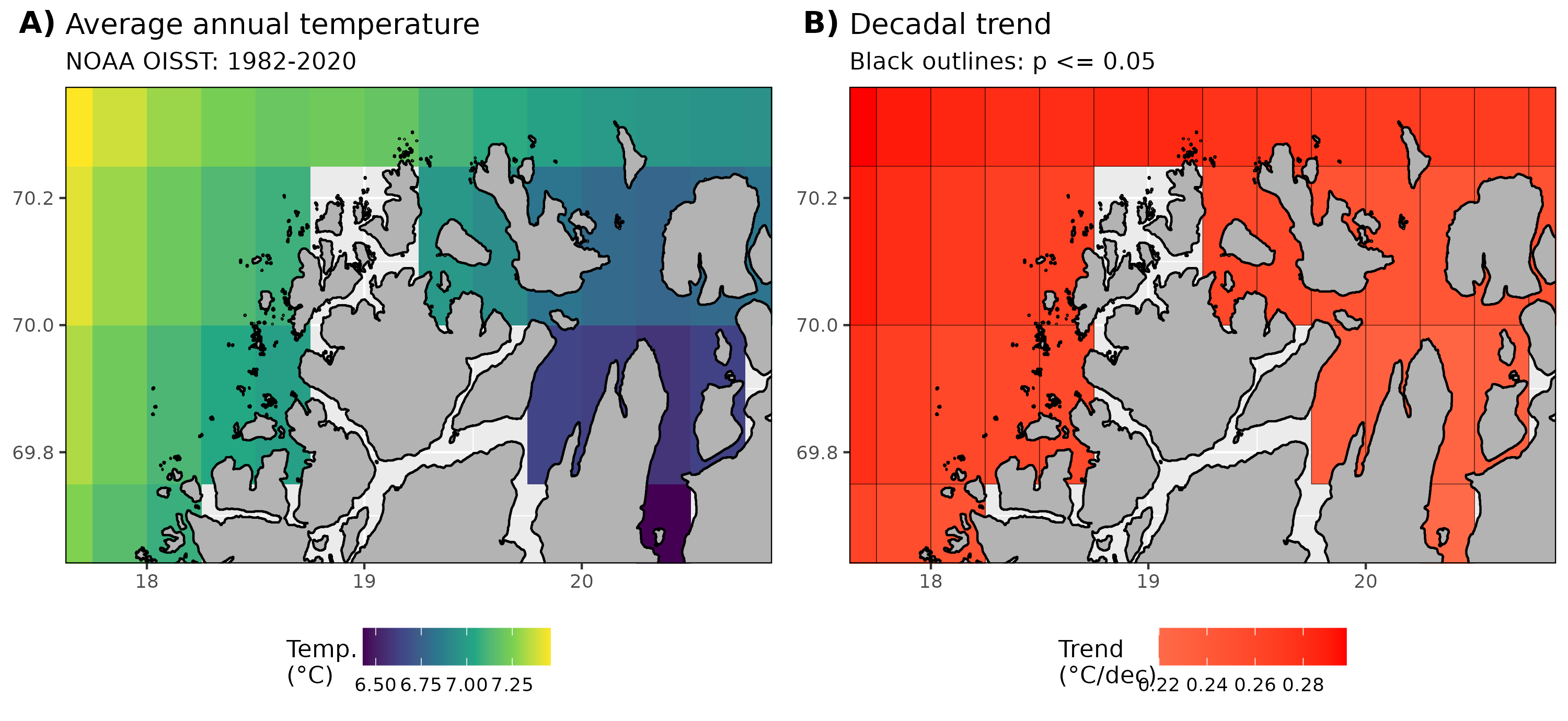
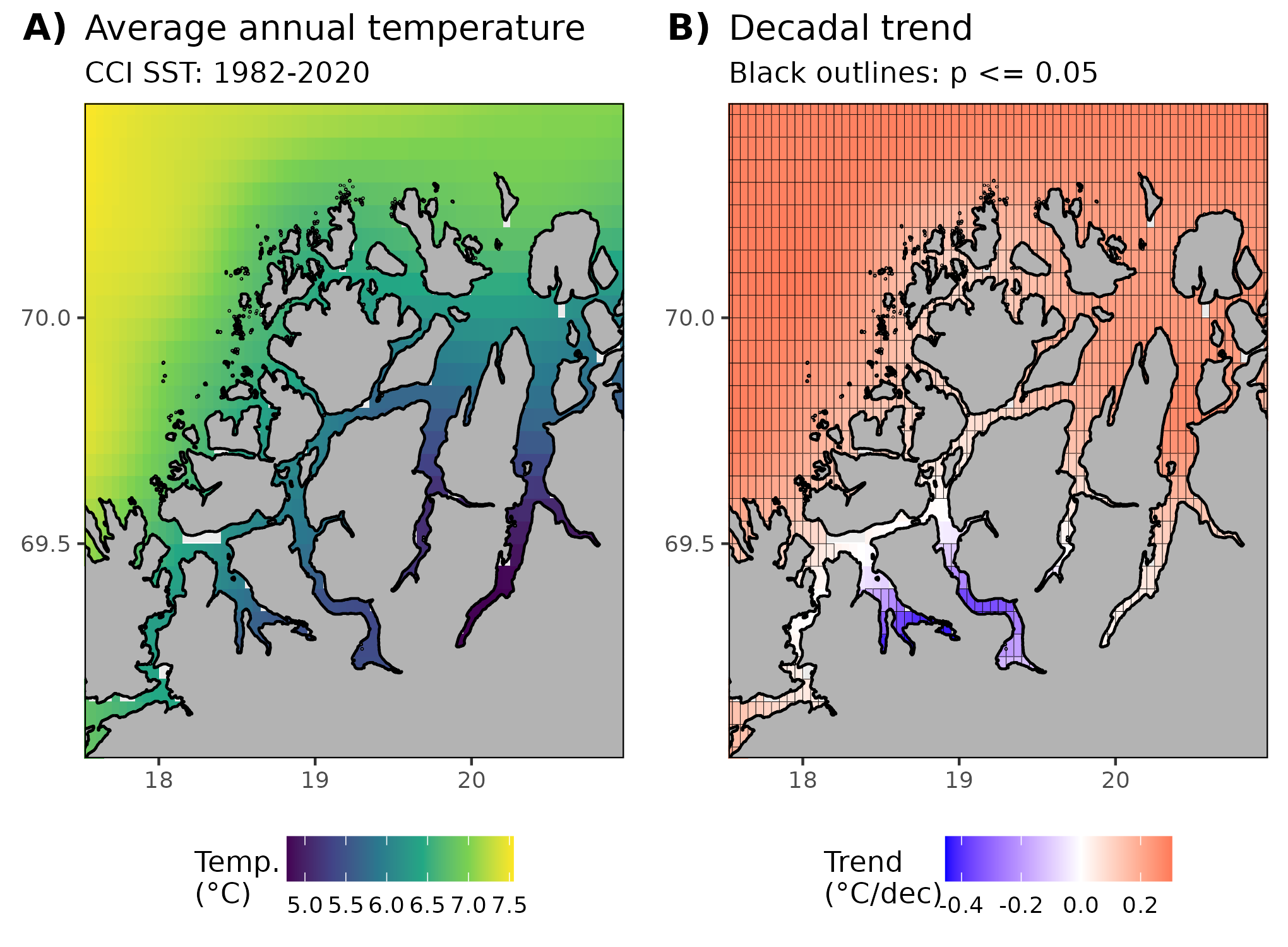
This document contains a summary of the NOAA OISST, CCI SST (sea surface temperature), and model data that have been extracted around the FACE-IT sites. Both satellite products have daily data from 1982 to 2020 however, the NOAA data are on a 0.25° grid while the CCI data are at 0.05°. This difference in the size of the pixels allows for some dramatic differences int he observed temperatures along the coast and in the fjords, as well as the decadal trends of those temperatures. Most importantly, the NOAA pixels are too coarse to capture SST within most of the FACE-IT fjords while CCI is able to provide SST in all sites. The coastal/fjord pixels in the CCI data also tend to show strong cooling trends. I assume that these cooling trends are an artefact of the increased glacial melting into the fjord. But we can’t rule out that they are caused by any of the common remotely sensed coastal pixel issues, such as land bleed, which can interfere with the accurate assimilation of the data. Regardless, even in the more open coastal waters these two products do not agree very closely with one another and this is cause for some alarm. It is known that remotely sensed products begin to differ significantly from one another when approaching the poles and the quick analysis performed here certainly confirms that once again.

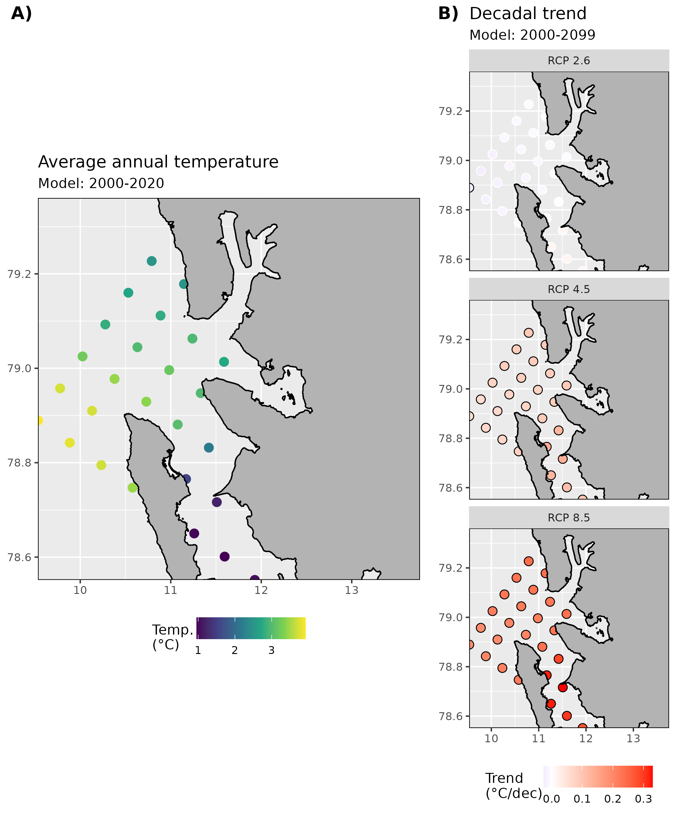
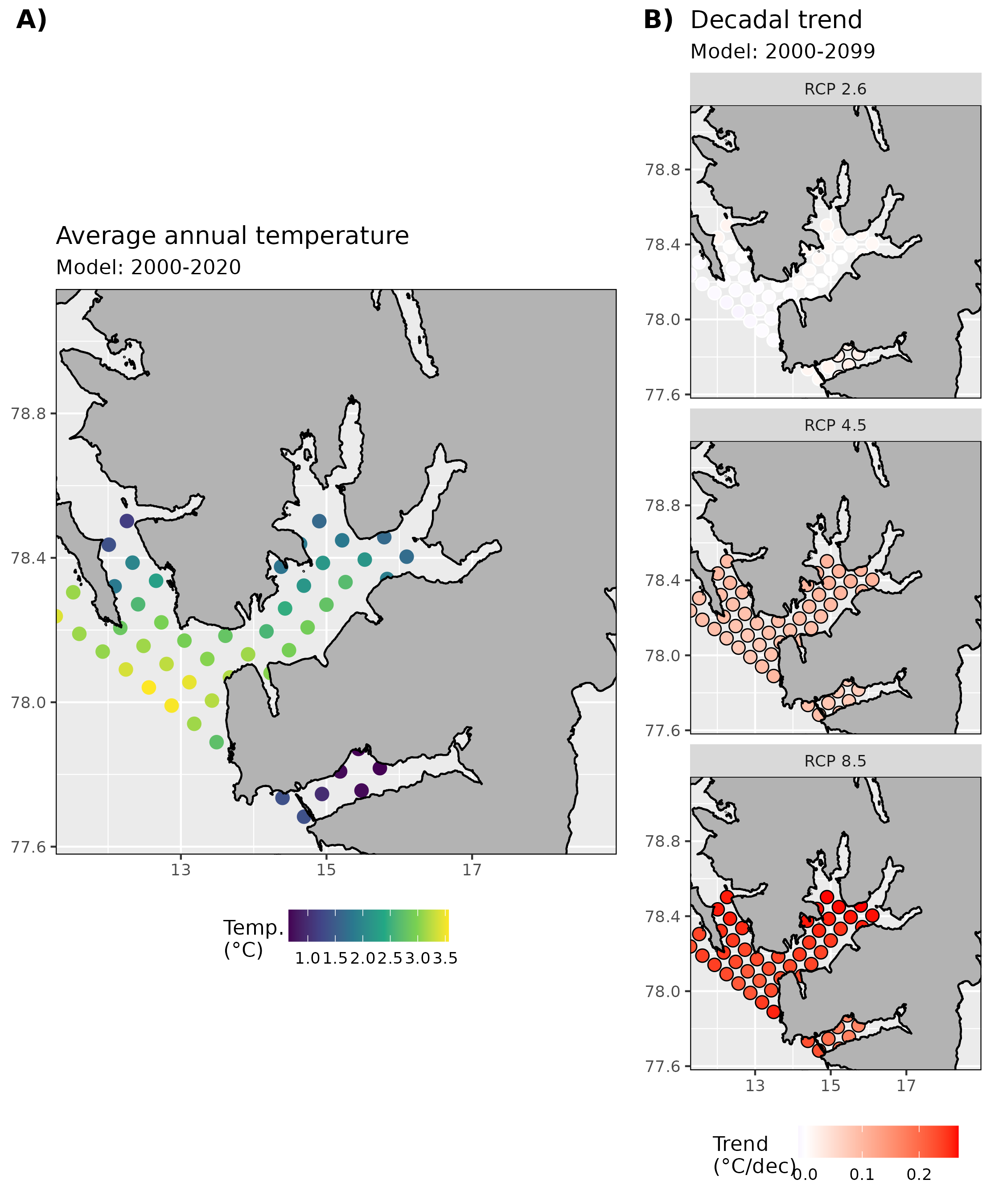
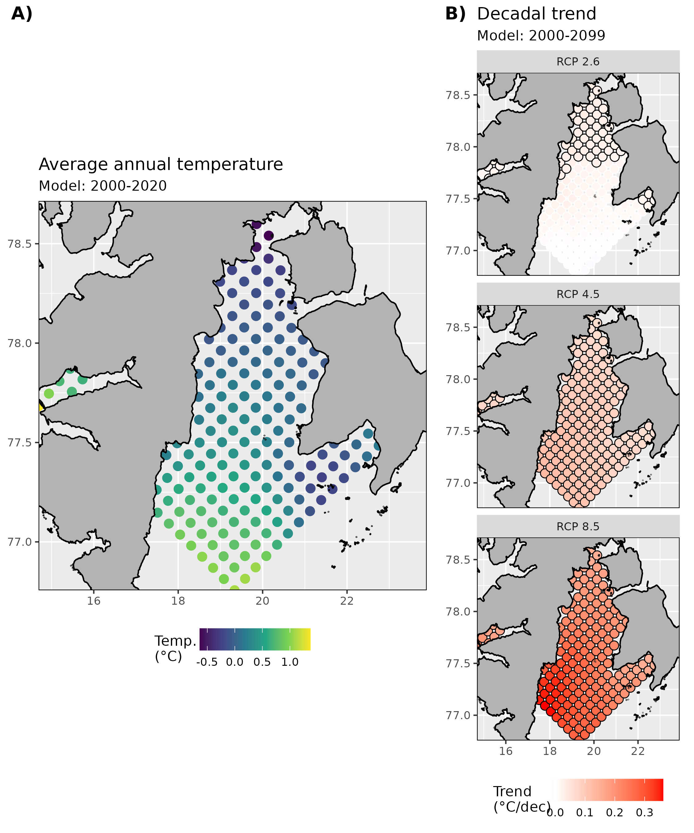
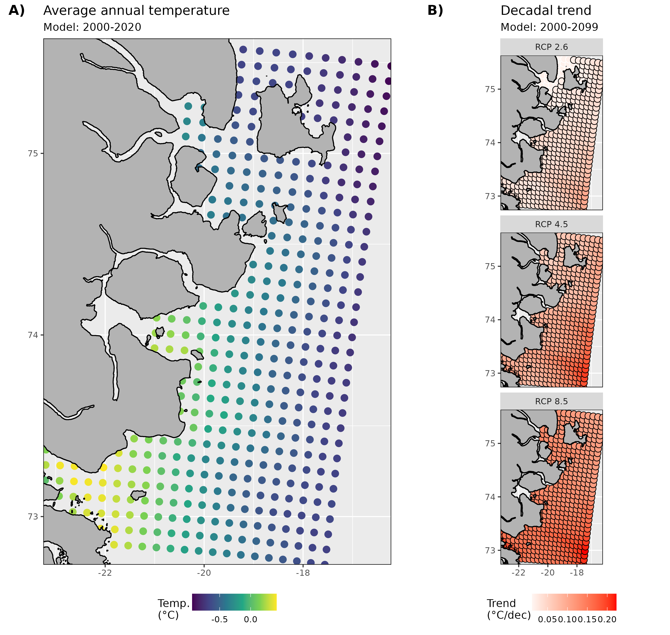
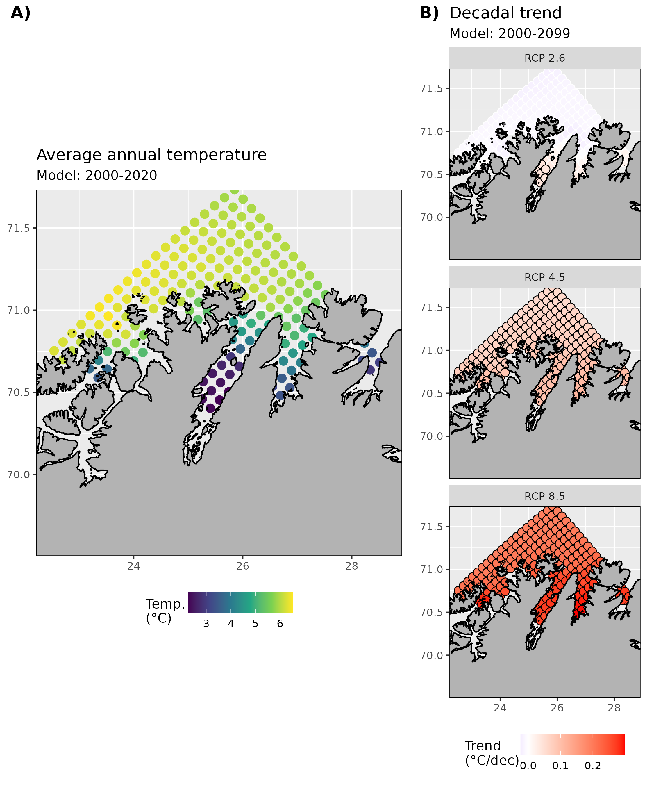
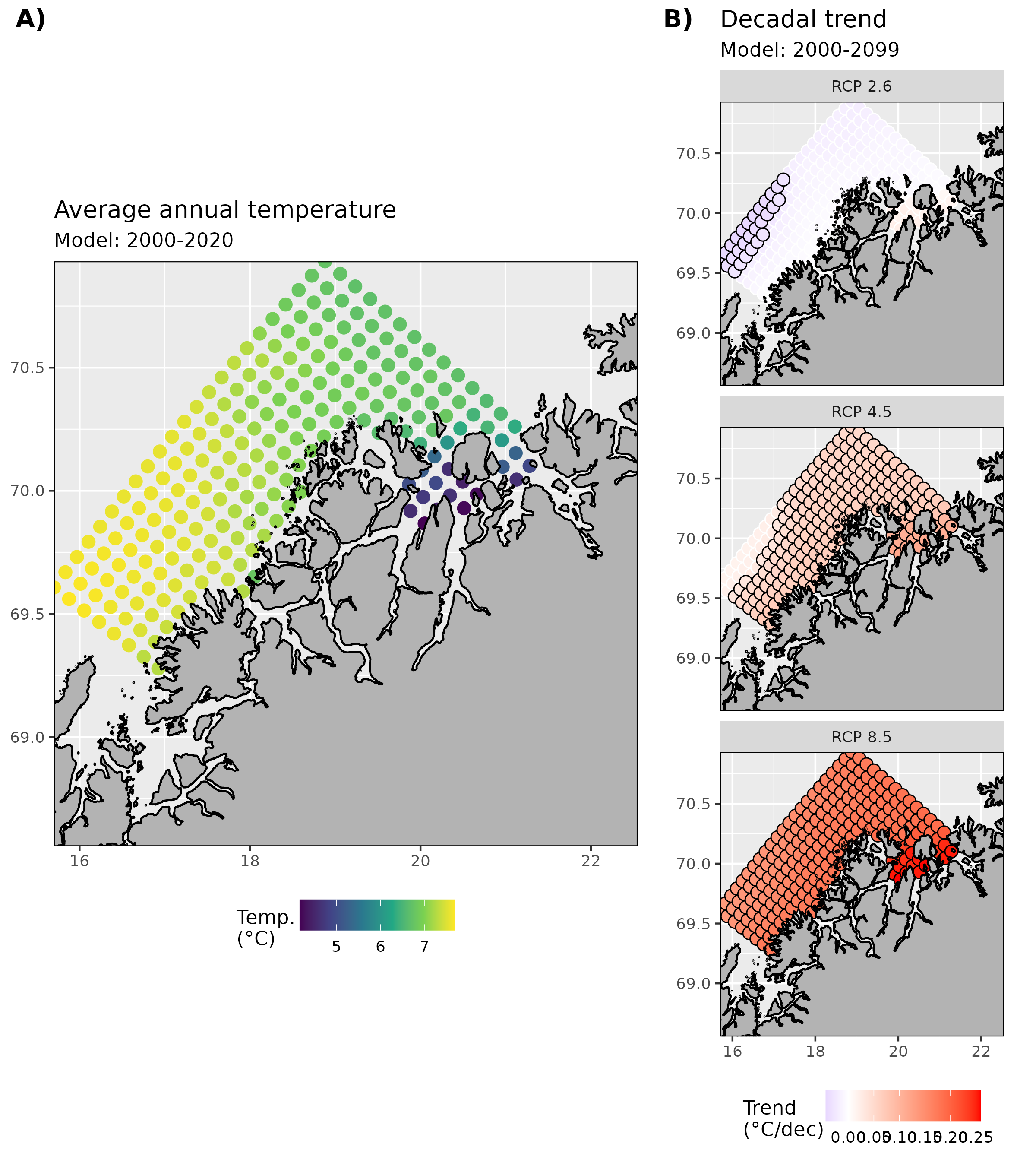
The model data used here run from 2000-2099 and area available for three different climate pathways (RCP: 2.6, 4.5, 8.5) and at multiple depths (0, 50, 100, 200 m). The model is not generated on a Cartesian coordinate system so the values are shown as points, rather than as a raster. The model projections for RCP 8.5 tend to produce decadal trends that are similar to the NOAA OISST trends, implying that the current pathway we are on is 8.5, which matches most of the past literature, but moving forward we may be coming closer to RCP 7.0. Note also that the present day SST values between the model and the NOAA OISST values tend to match ore closely than to the CCI SST.

The rest of this page provides the results of the analysis by FACE-IT site. One may use the table of contents on the left to jump to a desired section. Each figure shown here has two panels: A) The average temperatures from 1982-2020, and B) The decadal trend over the same period. The first figure shows the results from the NOAA OISST data, the second for the CCI SST data, and the third for the model. Note that the model was not run for the western side of Greenland so there are no data available for Disko Bay or Nuup Kangerlua.

Svalbard

Kongsfjorden

Figure 1: A) Average annual SST from 1982-2020. B) Decadal trends in SST calculated with annual averages from 1982-2020. Pixels with significant trends (p <= 0.05) are framed in black. Note that the pixels in the NOAA OISST product are ~25km so there are no data within Kongsfjorden. One must also be cautious of the effect of land bleed on the temperatures for pixels that contain coastline.
Figure 2: A) Average annual SST from 1982-2020. B) Decadal trends in SST calculated with annual averages from 1982-2020. Pixels with significant trends (p <= 0.05) are framed in black. Note that the pixels in the CCI SST product are ~5km so there are data within Kongsfjorden. How exactly these data points came to exist is curious and one should maintain a healthy skepticism of these results.
Figure 3: A) Average annual SST from 2000-2020. B) Decadal trends in SST calculated with annual averages from 2000-2099. Decadal trends are shown for the three most commonly used RCPs. Pixels with significant trends (p <= 0.05) are framed in black. Note that the pixels in the model product are not on a cartesian grid so are shown here as points rather than as a raster.

Isfjorden

Figure 4: A) Average annual SST from 1982-2020. B) Decadal trends in SST calculated with annual averages from 1982-2020. Pixels with significant trends (p <= 0.05) are framed in black.
Figure 5: A) Average annual SST from 1982-2020. B) Decadal trends in SST calculated with annual averages from 1982-2020. Pixels with significant trends (p <= 0.05) are framed in black.
Figure 6: A) Average annual SST from 2000-2020. B) Decadal trends in SST calculated with annual averages from 2000-2099. Decadal trends are shown for the three most commonly used RCPs. Pixels with significant trends (p <= 0.05) are framed in black.

Storfjorden

Figure 7: A) Average annual SST from 1982-2020. B) Decadal trends in SST calculated with annual averages from 1982-2020. Pixels with significant trends (p <= 0.05) are framed in black.
Figure 8: A) Average annual SST from 1982-2020. B) Decadal trends in SST calculated with annual averages from 1982-2020. Pixels with significant trends (p <= 0.05) are framed in black.
Figure 9: A) Average annual SST from 2000-2020. B) Decadal trends in SST calculated with annual averages from 2000-2099. Decadal trends are shown for the three most commonly used RCPs. Pixels with significant trends (p <= 0.05) are framed in black.

Greenland

Young Sound

Figure 10: A) Average annual SST from 1982-2020. B) Decadal trends in SST calculated with annual averages from 1982-2020. Pixels with significant trends (p <= 0.05) are framed in black.
Figure 11: A) Average annual SST from 1982-2020. B) Decadal trends in SST calculated with annual averages from 1982-2020. Pixels with significant trends (p <= 0.05) are framed in black.
Figure 12: A) Average annual SST from 2000-2020. B) Decadal trends in SST calculated with annual averages from 2000-2099. Decadal trends are shown for the three most commonly used RCPs. Pixels with significant trends (p <= 0.05) are framed in black.

Disko Bay

Figure 13: A) Average annual SST from 1982-2020. B) Decadal trends in SST calculated with annual averages from 1982-2020. Pixels with significant trends (p <= 0.05) are framed in black.
Figure 14: A) Average annual SST from 1982-2020. B) Decadal trends in SST calculated with annual averages from 1982-2020. Pixels with significant trends (p <= 0.05) are framed in black.

Nuup Kangerlua

Figure 15: A) Average annual SST from 1982-2020. B) Decadal trends in SST calculated with annual averages from 1982-2020. Pixels with significant trends (p <= 0.05) are framed in black.
Figure 16: A) Average annual SST from 1982-2020. B) Decadal trends in SST calculated with annual averages from 1982-2020. Pixels with significant trends (p <= 0.05) are framed in black.

Norway

Porsangerfjorden

Figure 17: A) Average annual SST from 1982-2020. B) Decadal trends in SST calculated with annual averages from 1982-2020. Pixels with significant trends (p <= 0.05) are framed in black.
Figure 18: A) Average annual SST from 1982-2020. B) Decadal trends in SST calculated with annual averages from 1982-2020. Pixels with significant trends (p <= 0.05) are framed in black.
Figure 19: A) Average annual SST from 2000-2020. B) Decadal trends in SST calculated with annual averages from 2000-2099. Decadal trends are shown for the three most commonly used RCPs. Pixels with significant trends (p <= 0.05) are framed in black.

Tromsø

Figure 20: A) Average annual SST from 1982-2020. B) Decadal trends in SST calculated with annual averages from 1982-2020. Pixels with significant trends (p <= 0.05) are framed in black.
Figure 21: A) Average annual SST from 1982-2020. B) Decadal trends in SST calculated with annual averages from 1982-2020. Pixels with significant trends (p <= 0.05) are framed in black.
Figure 22: A) Average annual SST from 2000-2020. B) Decadal trends in SST calculated with annual averages from 2000-2099. Decadal trends are shown for the three most commonly used RCPs. Pixels with significant trends (p <= 0.05) are framed in black.

R version 4.3.3 (2024-02-29)
Platform: x86_64-pc-linux-gnu (64-bit)
Running under: Ubuntu 20.04.6 LTS

Matrix products: default
BLAS:   /usr/lib/x86_64-linux-gnu/openblas-pthread/libblas.so.3 
LAPACK: /usr/lib/x86_64-linux-gnu/openblas-pthread/liblapack.so.3;  LAPACK version 3.9.0

locale:
 [1] LC_CTYPE=en_GB.UTF-8       LC_NUMERIC=C              
 [3] LC_TIME=en_GB.UTF-8        LC_COLLATE=en_GB.UTF-8    
 [5] LC_MONETARY=en_GB.UTF-8    LC_MESSAGES=en_GB.UTF-8   
 [7] LC_PAPER=en_GB.UTF-8       LC_NAME=C                 
 [9] LC_ADDRESS=C               LC_TELEPHONE=C            
[11] LC_MEASUREMENT=en_GB.UTF-8 LC_IDENTIFICATION=C       

time zone: UTC
tzcode source: system (glibc)

attached base packages:
[1] stats     graphics  grDevices utils     datasets  methods   base     

other attached packages:
[1] workflowr_1.7.1

loaded via a namespace (and not attached):
 [1] vctrs_0.6.5       httr_1.4.7        cli_3.6.2         knitr_1.45       
 [5] rlang_1.1.3       xfun_0.41         stringi_1.8.3     processx_3.8.3   
 [9] promises_1.2.1    jsonlite_1.8.8    glue_1.7.0        rprojroot_2.0.4  
[13] git2r_0.33.0      htmltools_0.5.7   httpuv_1.6.14     ps_1.7.6         
[17] sass_0.4.8        fansi_1.0.6       rmarkdown_2.25    jquerylib_0.1.4  
[21] tibble_3.2.1      evaluate_0.23     fastmap_1.1.1     yaml_2.3.8       
[25] lifecycle_1.0.4   whisker_0.4.1     stringr_1.5.1     compiler_4.3.3   
[29] fs_1.6.3          pkgconfig_2.0.3   Rcpp_1.0.12       rstudioapi_0.15.0
[33] later_1.3.2       digest_0.6.34     R6_2.5.1          utf8_1.2.4       
[37] pillar_1.9.0      callr_3.7.3       magrittr_2.0.3    bslib_0.6.1      
[41] tools_4.3.3       cachem_1.0.8      getPass_0.2-4